INTEREST-RATE MODELS FOR US AND UK WITH MIXED INFLATIONARY EXPECTATIONS. A COMPARISON WITH THE RATIONAL AND THE
ADAPTATIVE SCHEME*
MaMar Sánchez
WP-AD 2002-05
Correspondence: University of Alicante, Facultad de Economics, Depto. de Funda- mentos del Análisis Económico, Ctra. San Vicente del Raspeig, s/n. 03071 (Alicante, Spain). Tel.: 96 590 36 14 / Fax: 96 590 36 85 / E-mail: [email protected].
Editor: Instituto Valenciano de Investigaciones Económicas, S.A.
First Edition June 2002.
Depósito Legal: V-2065-2001
IVIE working papers offer in advance the results of economic research under way in order to encourage a discussion process before sending them to scientific journals for theirfinal publication.
* The author wishes to express her gratitude to Ignacio Mauleón for his invaluable help, as well as to Juan Mora and an anonymous referee from the Ivie for their helpful comments and suggestions. Any remaining errors are the sole responsibility of the author. Financial support from the Spanish Government’s DGES (PB98-0979) grant is gratefully acknowledged.
INTEREST-RATE MODELS FOR US AND UK WITH MIXED INFLATIONARY EXPECTATIONS. A COMPARISON WITH
THE RATIONAL AND THE ADAPTATIVE SCHEME M
aMar Sánchez
A B S T R A C T
This paper presents a macro-econometric model for medium- and long-term nominal interest rates, assuming heterogeneous economic agents in the market that use different and limited sets of information. It also shows the empirical results obtained from US and UK data, comparing the performance of the model under mixed expectations with, respectively, the performance of the model under rational expectations and under a kind of adaptative expectation. The economet- ric problems arising in the mixed- and rational-expectation models are tackled by the generalized method of moments.
The mixed-expectation model picks up the dynamics of market expectations better than both the rationa-expectation model and the adaptative-expectation model, so that it provides the more reasonable model of interest-rate determina- tion.
Keywords: Interest-Rate Models, Mixed Expectations, Heterogeneous Agents, Rational Expectations, Adaptative Expectations, GMM Estimation.
1. INTRODUCTION
The determining of interest rates, a classical key issue in macro-economics, and the study of the formation of market-expectations, are the two main objectives of this paper.
The article is divided into two different parts. Thefirst is entirely theoretical and develops an explanatory model for the middle- and long-term nominal interest rate, assuming the existence of heterogeneous economic agents in the market who use different and limited pieces of information.
As in Mauleón and Sánchez (2000), our starting point is a sort of IS-LM-BP approach, in which the interest rate is considered to be the equilibrium price, from a global point of view, taking into account real, financial and foreign aspects, as well as the inter-dependence between the markets. Mixed expectations are assumed, however, for the expected inflation rate appearing in the explanatory equation for the nominal interest rate. The motivation is two-fold.
>From a theoretical point of view, the amount of information that economic agents are assumed to process in a rational-expectation model is unreasonably high. Furthermore, ignoring the speculative bubbles or explosive paths that some- times arise as a solution in this sort of model, implies using information that is not contained in the model.
>From an empirical point of view, there can be considerable divergences be- tween expected and observed inflation during certain periods, in which case, the use of actual inflation, instead of expected inflation, could yield rather imprecise estimators and produce systematic observed errors. Moreover, other explanatory variables of the model could proxy expected inflation if expectations are not cor- rectly measured.
In the second part of the paper, an empirical analysis for US and UK interest rates is carried out and the performance of the mixed-expectation model is studied and compared with the performance of the model under rational expectations and under a kind of adaptative expectation.
The remainder of this article is organised as follows. The following two sec- tions are purely theoretical and introduce the interest-rate model and the mixed- expectation mechanism. Sections 4 and 5 present the empirical analysis of the US and UK interest rates, respectively. Section 6 reviews the main results and offers the overall conclusions. Finally, an appendix provides information about the time-series employed.
2. THE INTEREST-RATE MODEL
There are two basic macro-economic models for determining interest rates: the savings market focus, which concentrates on the real aspects of the economy, and thefinancial approach, which includes the money market focus and the credit mar- ket focus. The latter is specially apt for explaining the influence of government deficits and foreign interest rates on the fixing of domestic interest rates. The loanable funds model, used by Hoelscher (1986) andCorreia-Nunes and Stemit- siotis (1995) among others, also studies the relationship between budget deficits and interest rates, explicitly considering the term structure of interest rates.
In this article, the evolution of medium- and long-term interest rates is anal- ysed within an eclectic model, covering financial, real and foreign aspects, in line with the global approach proposed by Mauleón (1991). The global approach is a three-market one (savings market, credit market and foreign market), and is equivalent to the IS-LM-BP approach1 in which the LM replaces the demand for credit.
As inRaymond and Mauleón (1997),and inMauleón and Sánchez (2000), the equilibrium condition of the savings market or the accounting identity between savings supply (SSt) and savings demand (SDt)
SSt =SDt (2.1)
is considered as a starting point, as it is equivalent to the equilibrium condition of the credit market and decisions on savings and investment are based on medium- and long-term considerations.
The equilibrium price, equating supply and demand for savings, is the real interest rate, which is defined as the nominal interest rate minus the expected inflation rate. The Uncovered Interest Rate Parity (the equilibrium condition in the international credit market under imperfect foresight), together with the Purchasing Power Parity (which holds for perfect arbitrage in the goods market), implies the international equalization of expected real interest rates in equilibrium (the Real Interest Rate Parity)2.
1See, for instance, Dornbusch and Fischer (1987) and the classical article ofHicks (1937), who introduced the IS-LM model.
2For instance, Wu and Chen (1998) examine the stationarity of real interest differentials and find empirical support for the Real Interest Rate Parity.
The savings supply is the sum of government, private and foreign savings.
Hereafter, government deficit, measured by real claims on government (RCt), is considered instead of government savings.
Private savings are assumed to depend on the nominal interest rate of domestic government bonds (Bt), on the expected national inflation rate (IRet), on the real volume of activity, measured by the real gross domestic product (RGDPt), on real money in the economy (RMt) and on real claims on government (RCt).
Foreign savings depend on the difference between the national nominal in- terest rate (Bt) and the foreign nominal interest rate (F Bt), as well as on the difference between the expected domestic inflation rate (IRet) and the expected foreign inflation rate (F IRet).
The resulting behavioural equation for the supply of savings during a given period t is given by Equation (2.2).
SSt=−RCt+a0+a1Bt−a2F Bt−a3IRte+a4F IRet+a5RGDPt+a6RMt+a7RCt+u1t
(2.2) The demand for savings or investment, defined by Equation (2.3), depends on the domestic nominal interest rate (Bt), on the share yield3 (SYt), on the expected inflation rate (IRet), on the real gross domestic product (RGDPt) and on real money4 (RMt).
SDt =b0−b1Bt+b2SYt+b3IRte+b4RGDPt+b5RMt+u2t (2.3) According to Tobin’s q scheme, investment increases when the ratio between the market value of stocks and their replacement cost, q, is greater than one. The market value of assets increases when the real interest rate decreases and when the real gross domestic product, the real money and the share yield increase. The replacement cost decreases when the real interest rate decreases and when the share yield increases: securing financial support is easier and cheaper for firms when the real interest rate decreases and when the growth rate of share prices increases.
3Also Knot (1995) introduces the share yield in his loanable funds model of investment demand, desired saving and net capital outflows.
4This kind of investment equation has been used before in Raymond and Mauleón (1997) and inMauleón and Sánchez (2000).
By substituting Equations (2.2) and (2.3) in the identity between supply and demand for savings and solving for the nominal interest rate, Equation (2.4) is obtained.
Bt=c0+c1F Bt+c2SYt+c3IRet−c4F IRet+c5RGDPt−c6RMt+c7RCt+u3t (2.4) This expresses the nominal interest rate as a function of the foreign interest rate, of the national and foreign expected inflation rates, of the real gross domestic product, of the real money, of the real claims on government and of the national share yield.
Note that considering nominal interest rates and expected inflation rates, rather than real interest rates, allows us to test the Fisher hypothesis or full translation of changes in inflation rates to nominal interest rates.
On the other hand, the significance of the variable “real claims on govern- ment” would imply that government deficits influence interest rates and that the Ricardian equivalence theorem should be rejected.
Finally, equation (2.4) may be made dynamic by including lags on both the domestic and foreign nominal interest rate, on the share yield, on the real GDP, on the real money and on the real claims on government. In fact, up to two lags are considered in the empirical work.
3. THE MIXED-EXPECTATION MECHANISM
A review of the evidence published on the formation of expectations shows that they are not rational: there is an up-date based on the recent past for short horizons and a certain persistence over the long run. Moreover, expectations are not consistent: the forward iteration of short-term expectations does not coincide with the observed long-term expectations. As such, we shall assume the existence of two different types of active agents in the market: fundamentalists and chartists.
The fundamentalists have the “regressive” expectations of long horizons. In other words, when a variable deviates from its equilibrium value, they expect that it will eventually return to its original value. They are rational agents, as they consided the information embodied in the structural model. They do not consider, however, the behaviour of the chartists in the market and the short-run dynamics
prompted by their behaviour5, so that they use a limited set of information.
Chartists, technical analysts or noise traders, consider all the relevant infor- mation about the behaviour of a variable to be reflected in its observed market values. Their information set is therefore different and limited as well. They detect patterns from the recent past of the variable and project them into the fu- ture, forming their expectations in an extrapolative manner, and thus, they tend to incorporate the “band-wagon effects” of short-term expectations.
Indeed, two expectations-generating mechanisms arise within the mixed-expectation scheme. The first one assumes that agents form their expectations in a model- consistent way. The second mechanism is a kind of adaptative expectation. Fur- thermore, as the fundamentalists and the chartists form their expectations in different ways, the forward iteration of the short-term expectation of the chartists does not match the long-term expectations of the fundamentalists.
The market’s expectation for the inflation rate (IRet) therefore includes the forecast made by the fundamentalists (IReft ) and the forecast made by the chartists (IRect ), in period t, with the information available at t-1. Note that all of the eco- nomic agents take their positions in the market in period t, based on their fore- casts, and that the market inflation rate in time t is not available to them when making decisions, as they use the information that is available at time t-1. For sufficiently short time-periods, the assumption on the timing of the information set is not very restrictive.
The weight of the two forecasts on the market’s expectations can be either constant or variable. Assuming a constant proportion of the fundamentalists (θ) and of the chartists (1−θ) in the market6, the expected inflation rate is given by the Equation (3.1).
IRet =θIReft + (1−θ)IRect , 0<θ<1 (3.1) When the weight of the fundamentalists (wt)and the weight of the chartists (1-
5This is also the definition of Frankel and Froot (1986) or De Grauwe, Dewachter and Em- brechts (1993), among others. Other authors, however, consider that the fundamentalists know both the structural model and the existence of chartists in the market, asMauleón (1996, 1998).
6See Mauleón (1996) and Mauleón (1998) for examples of a constant proportion of agents in the market.
wt)depend on market conditions7, the market’s expectation is given by Equation (3.2).
IRet =wtIReft + (1−wt)IRect , 0< wt<1 f or all t (3.2) The forecast made by the fundamentalists in period t will be a weighted av- erage of the r next inflation rates, for some r ∈N, since they form their expecta- tions in a model-consistent way and any future inflation rate expected by rational agents at time t is the conditional expectation for that inflation rate, based on the information set available to rational agents at time t-1.
IReft =φ(IRt+1, IRt+2, ..., IRt+r) (3.3) As we assume that the chartists extrapolate recent observed inflation rates into the future, the inflation rate expected by technical analysts at time t will be a function of s past values of the inflation rate, for some s ∈N.
IRect =ψ(IRt−s, IRt−s+1, ..., IRt−1) (3.4) Equation (3.4) is a general and easy way to describe the models used by the chartists, which can all be re-written as some weighted average of past values.
Finally, the variable market weight of the fundamentalists, is given by the following weighting function8.
wt= 1/(1 +δ(IRt−1−IRect−1)2) (3.5) When the market’s inflation rate at time t-1 equals the inflation rate expected by chartists for period t-1, the weight of the fundamentalists (wt) is one, as if there were only fundamentalists in the market. As the market rate deviates from its expected equilibrium value, chartists become more important and their weight on the market’s expectation (1−wt) tends to increase.
The parameterδdetermines the speed with which the weight of the fundamen- talists decreases or, put in another way, the speed with which the weight of the
7Frankel and Froot (1986) and De Grauwe, Dewachter and Embrechts (1993) also assume a variable proportion of agents in the market.
8This type of weighting function has been postulated before by De Grauwe, Dewachter and Embrechts (1993).
chartists increases. With a high “speed-parameter”, relatively small deviations of the market value from the inflation rate expected by the chartists lead to a great increase of the chartists influence in the market. This means that the estimates of the chartists are very precise, or that the variance of the equilibrium inflation rate expected by the chartists is small. As such,δ also measures the variability of the chartists estimates and will be defined here as the reciprocal of the variance of the chartists’ estimates, since, otherwise, the model becomes highly non-linear.
δ = 1/σ2IRec (3.6)
In the empirical analysis, σ2IRec is replaced by its unbiassed estimate:
s2IRec = (ΣTt=2(IRt−1−IRtec−1)2)/(T −2) (3.7)
4. EMPIRICAL RESULTS FOR U.S.
Let usairet be the variable market expectation about the US inflation rate in period t,
usairet =wtusaireft + (1−wt)usairect (4.1) where the inflation rate expected by fundamentalists in period t (usaireft ) is the next period inflation rate (as in the rational-expectation model),
usaireft =usairt+1 (4.2) and the inflation rate expected by chartists at time t (usairect ) is the inflation rate of period t-2 (the expected inflation rate obtained by lags selection in a model with adaptative expectations).
usairect =usairt−2 (4.3) The market weights of the fundamentalists and the chartists (wt and (1−wt) respectively) are defined accordingly, following Equations (3.5), (3.6), (3.7) and (4.3).
After deleting non-significant variables, such as the real claims on government, the share yield, the foreign (UK) interest rate, the UK expected inflation rate, the constant term and some lags on other explanatory variables of the model, the
nominal interest rate of the US government bond reacts to changes in the lagged US interest rate, in the market’s expectations on the US inflation rate, in the US real money for the period t and t-1, and in the real US gross domestic product for t and t-1 (the real money and the real GDP are expressed in logarithms).
usabt = c1usabt−1+c2usairte+c3usarmt+c4usarmt−1+c5usargdpt+
c6usargdpt−1+vt (4.4)
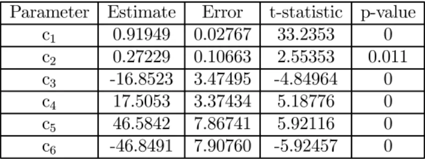
This explanatory equation is the same as the one obtained under rational expectations, except thatusairet is substituted by the t+1 inflation rate expected by fundamentalists during period t. To avoid the econometric problems derived from the correlation of the error term, with the regressors and with itself over time, Equation (4.4) is estimated by the generalized method of moments (GMM) using all the predetermined and weakly exogenous variables of the full-information model obtained for the US under rational expectations9as instruments: a constant, the lagged US interest rate, the US inflation rate for periods t-1, t-2 and t-3, the growth rate of the US nominal money for t-1, t-2, t-3, t-4, t-7 and t-8, the US real money for t and t-1, and the US real GDP for t and t-1. The results are given in Table 1.
TABLE 1: GMM estimation of the US interest-rate model with a variable proportion of heterogeneous agents in the market.
Parameter Estimate Error t-statistic p-value c1 0.91949 0.02767 33.2353 0 c2 0.27229 0.10663 2.55353 0.011 c3 -16.8523 3.47495 -4.84964 0 c4 17.5053 3.37434 5.18776 0 c5 46.5842 7.86741 5.92116 0 c6 -46.8491 7.90760 -5.92457 0
Notes: Standard Errors computed from heteroscedastic-consistent matrix (Robust-White) also robust to autocorrelation (NMA= 2, Kernel=Bartlett). E’HH’E (the objective function for
9SeeMauleón and Sánchez (2000) for further details.
the gmm estimation, evaluated from the solution) = 0.13015. Test of overidentifying restric- tions = 12.4940 [0.187]. Degrees of freedom = 9. Adjusted R-squared = 0.94770. Number of Observations = 96. Current sample: 1974:1 to 1997:4.
It is worthwhile remarking that the GMM estimation of the model with a constant proportion of heterogeneous agents in the market, equal to the mean of the market weights (0.68223 for the fundamentalists and 0.31777 for the chartists), yields a similar outcome, so that we only present and comment on the results obtained from the model with variable market weights.
The estimated coefficient for thefirst lag of the US bond shows a good deal of inertia, although is not very close to one. The real claims on the US government is non-significant, which implies that the coefficienta7 in the savings supply equation is equal to one: the US private sector fully compensates for the prodigality of the government and vice versa, so that increments in the government deficit do not affect the interest rate and the Ricardian equivalence theorem is fulfilled.
The share yield is also non-significant, either because the nominal interest rate influences the share yield and not the other way around, or because the two financial variables are determined by real variables in spite of being mutually related.
Finally, note that the estimated coefficients of real money for period t and for period t-1 are very close in absolute value, but with a different sign. And the same thing happens with the estimated coefficients of real GDP for period t and t-1. Considering that real money and real GDP are expressed in logarithms, we accept that the explanatory variables are the growth rate of real money and the growth rate of real GDP and estimate Equation (4.4) again, with the restrictions c4 =−c3 andc6 =−c5.
Next, restrictions are also imposed on Equation (4.4) with the aim of obtaining the estimated coefficients in the dynamic equilibrium.
c?2 = c2/((1−c1)×4)
c?3 = (c3+c5)/((1−c1)×400)
On the one hand, regardless of the expectation scheme assumed, all economic agents in the market are rational in equilibrium and thus the expected inflation
rate is equal to the observed inflation rate. On the other hand, since only the interest rate is expressed in per cent per annum, the coefficients of the other quarterly variables have to be divided by four. Besides, the coefficients of the increment of real GDP and of the increment of real money have to be divided by 100 to get the coefficients of the corresponding growth rates in percentages.
Lastly, we assume that the nominal interest rate is constant through time and that real money and real gross domestic product grow at the same rate in equilibrium.
The result is that only the US inflation rate and the growth rate of the US real GDP influence the nominal interest rate of the US government bond in dynamic equilibrium, as Equation (4.5) shows.
usabt = 0.72715 usairt+ 1.10111 ∆usargdpt (4.5) Note that the estimated coefficient of the inflation rate is quite high, even though the Fisher hypothesis is not completely fulfilled. This means that the inflation rate is important for controlling the nominal interest rate, that finan- cial markets are rather efficient (economic agents are relatively well-informed and transaction costs are not very high), and that real interest rates are important when decisions are made (which supports the choice of the theoretical approach used to develop the model).
Finally, if the Fisher hypothesis were completely fulfilled, the real interest rate would be determined by the growth rate of real GDP in equilibrium.
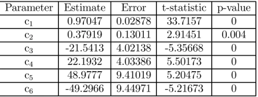
According to Table 2, the results from the GMM estimation of the above mixed-expectation model are very close to those from the GMM estimation of the rational-expectation model defined by Equation (4.6).
usabt = c1usabt−1+c2usairt+1+c3usarmt+c4usarmt−1+c5usargdpt+
c6usargdpt−1+vt (4.6)
TABLE 2: GMM estimation of the US interest-rate model with rational infla- tionary expectations.
Parameter Estimate Error t-statistic p-value c1 0.91580 0.02854 32.0904 0 c2 0.33347 0.14765 2.25859 0.024 c3 -13.0706 4.63002 -2.8230 0.005 c4 14.1544 4.30727 3.28615 0.001 c5 42.5846 7.77777 5.47517 0 c6 -43.0308 7.82038 -5.50238 0
Notes: Standard Errors computed from heteroscedastic-consistent matrix (Robust-White) also robust to autocorrelation (NMA= 1, Kernel=Bartlett). E’HH’E = 0.11705. Test of over- identifying restrictions = 11.2363 [0.260]. Degrees of freedom = 9. Adjusted R-squared = 0.94694. Number of Observations = 96. Current sample: 1974:1 to 1997:4.
Equation (4.6) is estimated again with the restrictionsc4 =−c3 andc6 =−c5, which are also accepted for this model. Then, the restrictions below are imposed on the new model to obtain the estimated coefficients in equilibrium, substituting the observed inflation rate for the expected inflation rate and assuming that the nominal interest rate is constant over time and that the growth rate of real money is equal to the growth rate of real GDP.
c?2 = c2/((1−c1)×4)
c?3 = (c3+c5)/((1−c1)×400)
The nominal interest rate, in equilibrium, is given by Equation (4.7) and, according to it, the rational-expectation model works a little better than the mixed-expectation model with regard to the Fisher hypothesis.
usabt = 0.76461usairt+ 1.04415∆usargdpt (4.7)
Finally, Table 3 shows the results from the OLS estimation of the model under a kind of adaptative expectation, according to the specification given by:
usabt = c1usabt−1+c2usairtec+c3usarmt+c4usarmt−1+c5usargdpt+
c6usargdpt−1+vt (4.8)
TABLE 3: OLS estimation of the US interest-rate model with a kind of adap- tative inflationary expectation.
Parameter Estimate Error t-statistic p-value c1 0.97047 0.02878 33.7157 0 c2 0.37919 0.13011 2.91451 0.004 c3 -21.5413 4.02138 -5.35668 0 c4 22.1932 4.03386 5.50173 0 c5 48.9777 9.41019 5.20475 0 c6 -49.2966 9.44971 -5.21673 0
Notes: Standard Errors are heteroskedastic-consistent10. Durbin’s h = -0.52750 [0.598].
Durbin’s h alt. = -0.56304 [0.573]. Sum of squared residuals= 31.5164. Jarque-Bera test = 2.84257 [0.241]. Ramsey’s RESET2 = 6.11070 [0.015]. F (zero slopes) = 335.710 [0]. R-squared
= 0.94911. Schwarz B.I.C. =-0.82857. Adjusted R-squared = 0.94629. LM het. test = 5.10582 [0.024]. Number of Observations = 96. Current sample: 1974:1 to 1997:4.
Note that the estimated coefficient of the lagged nominal interest rate (the estimated value of c1) is quite high. Moreover, the functional form of the linear regression model estimated seems to be incorrect, according to Ramsey’s RESET2 test, and the residual variances seem to be heteroscedastic, according to the LM heteroscedasticity test. These two results could be due to the omission of relevant variables in the above specification or to an incorrect dynamic specification, caused by the wrong measurement of market expectations. Hence we shall treat the results of subsequent analysis with caution.
10The variance-covariance matrix estimate has the form V=(X´X)−1X´diag(e2i/di)X (X´X)−1, where di=1-hi if hi=diag(X(X´X)−1X´)6= 1 for all i, and di=(T-k)/T if hi=1 for some i. This is a modified version of the White’s estimate, with betterfinite-sample properties than the estimate proposed by White (1980). See section 16.3 of Davidson and Mackinnon (1993) for more details.
>From a statistical point of view, and according to the adjusted R-squared values, the best model is the interest-rate model with mixed expectations, and the worst is the model with adaptative expectations.
Since we accept that c4 = −c3 and also that c6 = −c5, we estimate the re- stricted model and, afterwards, calculate the estimated coefficients in equilibrium, where the expected inflation rate is equal to the observed inflation rate, assuming the same nominal interest rate in period t and t-1, and the same growth rate for real money and real GDP.
c?2 = c2/((1−c1)×4)
c?3 = (c3+c5)/((1−c1)×400)
This procedure yields Equation (4.9).
usabt= 1.14usairt+ 0.7888∆usargdpt (4.9) Now, the nominal interest rate is more sensitive to the inflation rate than expected according to the Fisher effect. This is the Darby effect, which can occur when economic agents consider that the real after-tax interest rate is the relevant one. This argument is at odds with the theoretical model of real interest rate determination, developed in this article, as well as with the empirical evidence provided by the mixed- and rational-expectation models. Furthermore, in the literature, the empirical evidence in favour of the Darby effect is very limited.
Considering the above statistical and economic arguments, the interest-rate model obtained under a kind of adaptative expectation seems to be not very reasonable.
5. EMPIRICAL RESULTS FOR U.K.
Let ukirte be the variable market expectation of the UK inflation rate,
ukiret =wtukirtef + (1−wt)ukirtec (5.1) where the inflation rate expected by fundamentalists in period t (ukireft ) is, after analysing the performance of different alternatives, a weighted average of the next two UK inflation rates,
ukireft = (ukirt+1+ukirt+2)/2 (5.2) and the inflation rate expected by technical analysts at time t (ukirect ) is a weighted average of the past three UK inflation rates (the expected inflation rate that yields the best fit in a model with adaptative expectations).
ukirtec = 1/3 ukirt−1+ 1/3 ukirt−2+ 1/3 ukirt−3 (5.3) The UK market weights, wt and(1−wt), are generated according to Equations (3.5), (3.6), (3.7) and (5.3).
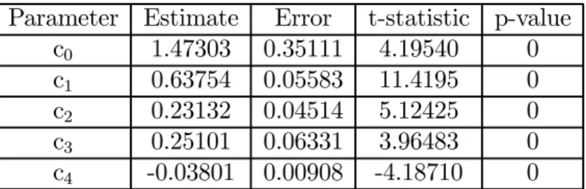
After deleting non-significant explanatory variables, the UK nominal interest rate depends on a constant term, on the lagged UK interest rate, on the US nominal interest rate, on the UK inflationary market expectation and on the UK share yield.
ukbt=c0+c1ukbt−1+c2usabt+c3ukirte+c4uksyt+vt (5.4) This equation is estimated by GMM with the proper instruments, which are all the predetermined and weakly exogenous variables of the full-information model that we would have obtained by modelling the UK inflation rate for t+1 and t+2 under rational expectations: a constant, the lagged UK interest rate, the UK inflation rate for period t-1, t-2, t-3 and t-4, the UK unit labor cost for t-1 and t-2, the US nominal interest rate, and the UK share yield. Table 4 shows the results.
TABLE 4: GMM estimation of the UK interest-rate model with a variable proportion of heterogeneous agents in the market.
Parameter Estimate Error t-statistic p-value c0 1.47303 0.35111 4.19540 0 c1 0.63754 0.05583 11.4195 0 c2 0.23132 0.04514 5.12425 0 c3 0.25101 0.06331 3.96483 0 c4 -0.03801 0.00908 -4.18710 0
Notes: Standard Errors computed from heteroscedastic-consistent matrix (Robust-White) also robust to autocorrelation (NMA= 1, Kernel=Bartlett). E’HH’E = 0.02003. Test of overi- dentifying restrictions = 1.90274 [0.862]. Degrees of freedom = 5. Adjusted R-squared = 0.89218. Number of Observations = 95. Current sample: 1974:1 to 1997:3.
The GMM estimation of the mixed-expectation model with a proportion of the fundamentalists and of the chartists equal to the mean of the respective market weights (0.67187 and 0.32813) produces similar results. Hence, only the results from the model with a variable proportion of agents in the market are reported.
As Table 4 shows, the estimated coefficient of the lagged national interest rate is far from one, denoting less inertia than in the case of the US.
The non-significance of the real claims on the UK government supports the Ricardian hypothesis, which is theoretically compatible with the middle- and long- run interest-rate model developed.
The nominal interest rate depends on the foreign interest rate: the US nominal interest rate influences the UK nominal interest rate, but the reverse is not true as the empirical results in the previous section show. This is only to be expected due to the size and economic leadership of the United States.
Eventually, the yield of the UK bond decreases by 3.8% when the UK share yield increases, which can be interpreted as a modest short-term portfolio re- allocation and as a spurious correlation in equilibrium, since the influence of the share yield on the nominal interest rate should be positive and higher.
In equilibrium, the expected inflation rate equals the observed inflation rate, the UK nominal interest rate is assumed to be constant over time and the UK inflation rate is assumed to be equal to the US inflation rate. Disregarding the equilibrium effect of the UK share yield and considering the equilibrium effect of the US inflation rate and real GDP on the foreign (US) nominal interest rate obtained from the US mixed-expectation model, the following restrictions are imposed on Equation (5.4) to achieve the annual estimated coefficients in the dynamic equilibrium.
c?0 = c0/(1−c1)
c?2 = (c2/((1−c1)×4))) + ((c3×0.72715)/(1−c1)) c?3 = (c3×1.10111)/(1−c1)
According to Equation (5.5), the UK nominal interest rate varies with the US nominal interest rate in dynamic equilibrium.
ukbt= 4.06397 + 0.63719 usairt+ 0.70272∆usargdpt (5.5)
The estimated coefficient of the inflation rate in equilibrium is lower than in the case of the US and, if the Fisher hypothesis were completely fulfilled, about 70% of the change in the growth rate of the real GDP would translate to the real interest rate.
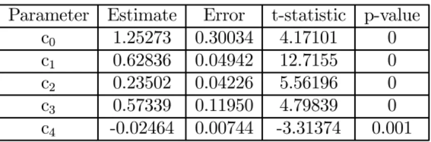
Next, Table 5 presents the results from the GMM estimation of the rational- expectation model obtained for the UK and defined by Equation (5.6).
ukbt=c0+c1ukbt−1+c2usabt+c3usairt+2+c4uksyt+vt (5.6)
TABLE 5: GMM estimation of the UK interest-rate model with rational in- flationary expectations.
Parameter Estimate Error t-statistic p-value c0 1.25273 0.30034 4.17101 0 c1 0.62836 0.04942 12.7155 0 c2 0.23502 0.04226 5.56196 0 c3 0.57339 0.11950 4.79839 0 c4 -0.02464 0.00744 -3.31374 0.001
Notes: Standard Errors computed from heteroscedastic-consistent matrix (Robust-White) are also robust to autocorrelation (NMA= 1, Kernel=Bartlett). E’HH’E = 0.06061. Test of over-identifying restrictions = 5.7583 [0.764]. Degrees of freedom = 9. Adjusted R-squared = 0.88240. Number of Observations = 95. Current sample: 1974:1 to 1997:3.
The results from the GMM estimation of the UK mixed-expectation model are better than those from the GMM estimation of the UK rational-expectations model. On the one hand, the value of the objective function in the solution is lower and the adjusted R-squared is higher. On the other hand, the UK nominal interest rate depends on the UK inflationary market expectation, rather than on the US expected inflation rate.
Even so, in equilibrium, the rational-expectation model works better than the mixed-expectation model, as can be seen from Equation (5.7).
ukbt= 3.37083 + 0.86926usairt+ 0.66032∆usargdpt (5.7)
This equation has been obtained by disregarding the influence of the UK share yield, by considering the rational-equilibrium effect of the US inflation rate and real GDP on the US nominal interest rate, as well as the equality between the expected and the observed inflation rate, and assuming that the UK nominal interest rate is constant in time and that the inflation rate of United States is equal to the inflation rate of United Kingdom in equilibrium. This implies estimating equation of (5.6) subject to the following restrictions.
c?0 = c0/(1−c1)
c?2 = (c2/((1−c1)×4))) + ((c3×0.76461)/(1−c1)) c?3 = (c3×1.04415)/(1−c1)
Finally, the results from the OLS estimation of the adaptative model defined by Equation (5.8) are reported in Table 6.
ukbt =c0+c1ukbt−1+c2usabt+c3ukirtec+c4uksyt+vt (5.8)
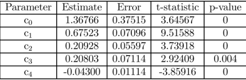
TABLE 6: OLS estimation of the UK interest-rate model with a kind of adap- tative inflationary expectation.
Parameter Estimate Error t-statistic p-value c0 1.36766 0.37515 3.64567 0 c1 0.67523 0.07096 9.51588 0 c2 0.20928 0.05597 3.73918 0 c3 0.20803 0.07114 2.92409 0.004 c4 -0.04300 0.01114 -3.85916 0
Notes: Standard Errors are heteroskedastic-consistent11. Durbin’s h = 2.40121 [0.016].
Durbin’s h alt. = 2.08608 [0.037]. Sum of squared residuals = 54.9975 Jarque-Bera test =
11The variance-covariance matrix estimate has the form V=(X´X)−1X´diag(e2i/di)X (X´X)−1, where di=1-hi if hi=diag(X(X´X)−1X´)6= 1 for all i, and di=(T-k)/T if hi=1 for some i. This is a modified version of the White’s estimate, with betterfinite-sample properties than the estimate proposed by White (1980). See section 16.3 of Davidson and Mackinnon (1993) for more details.
10.8155 [0.004]. Ramsey’s RESET2 = 2.83370 [0.096]. F (zero slopes) = 182.052 [0]. R-squared
= 0.888917. Schwarz B.I.C. = -0.31933. Adjusted R-squared = 0.88403. LM het. test = 3.39686 [0.065]. Number of Observations = 96. Current sample: 1974:1 to 1997:4.
>From a qualitative point of view, the mixed-expectation model and the adaptative-expectation model are better than the rational-expectation model, in- sofar as the UK nominal interest rate depends on the UK inflationary market expectation, rather than on the expected US inflation rate.
Note, however, that the null hypothesis of no autocorrelation is rejected in the model under a kind of adaptative expectation, according to Durbin’s h statistic.
The latter does not necessarily imply a problem of autocorrelation. Since the functional form of the linear regression model estimated is rejected according to Ramsey’s RESET2 test and the homoscedasticity of the residual variances is also rejected by the LM heteroscedasticity test, the problem could be the omission of relevant variables or an incorrect dynamic specification, asMaddala (1996)points out. Recall that we only consider the expectations of the chartists in this model and, as such, an important part of the market could have been ignored.
>From a quantitative point of view, the model under mixed expectations provides the best fit.
In order to reach the equilibrium expression for the UK nominal interest rate, Equation (5.8) is estimated again, substituting the observed inflation rate for the expected inflation rate, considering the effect of the US inflation rate and real GDP on the US nominal interest rate obtained from the US adaptative- expectation model, disregarding the UK share yield, and assuming that the UK nominal interest rate is constant in time and that the national inflation rate equals the foreign inflation rate.
c?0 = c0/(1−c1)
c?2 = (c2/((1−c1)×4))) + ((c3×1.14)/(1−c1)) c?3 = (c3×0.7888)/(1−c1)
The resulting Equation (5.9) shows that the UK nominal interest rate follows the US nominal interest rate and that, from the standpoint of the Fisher effect, the adaptative model works a little better than the rational-expectations model. In
any case, this equation has been calculated by considering the uncommon effect of the US inflation rate on the US nominal interest rate derived from the US adaptative-expectation model.
ukbt= 4.21115 + 0.89473 usairt+ 0.50829∆usargdpt (5.9)
6. SUMMARY AND CONCLUSIONS
This paper presents a theoretical model to explain the evolution of medium- and long-term nominal interest rates and gives empirical results obtained with US and UK data. Heterogeneous economic agents, with regard to inflation-rate expecta- tions, are assumed. The mixed-expectation model is analysed and compared to the rational-expectations model and to the adaptative-expectation model obtained for both the US and the UK nominal interest rates.
The theoretical framework is provided by a global approach, focusing on real, foreign andfinancial phenomena, and interest rates are thought to be determined by equilibrium in the savings market. This is equivalent to the credit market equilibrium.
In the explanatory equation for the nominal interest rate, the market infla- tionary expectation appears as a regressor, which is assumed to consist of the forecast made by fundamentalists, or rational agents, and the forecast made by chartists, or economic agents with a kind of adaptative expectation. The resulting model is estimated by GMM, to avoid the econometric problems that arise, and is compared to the GMM estimation of the model under rational expectations and the OLS estimation of the model under a kind of adaptative expectation.
Regardless of the expectation mechanism assumed, the US nominal interest rate depends on its first lag, on the expected US inflation rate and on the growth rates of real US money and real US GDP. The UK nominal interest rate depends on a constant term, on the lagged nominal UK interest rate, on the expected inflation rate and on the nominal US interest rate.
It is worthwhile remarking on the less than expected international integration offinancial markets, insofar as both national and foreign phenomena influence the nominal interest rate, and the fulfilment of the Ricardian equivalence theorem for the US and the UK, since government deficits are non-significant as expected in models of middle- and long-run interest-rate determination.
In equilibrium, the US nominal interest rate reacts to changes in the US infla- tion rate and in the growth rate of real US GDP, even if the Fisher hypothesis is not completely fulfilled. Indeed, if the Fisher hypothesis were fulfilled, the growth rate of the real GDP would determine the real interest rate.
The nominal UK interest rate follows the nominal US interest rate in the dynamic equilibrium.
The incomplete fulfilment of the Fisher hypothesis and the less than expected international integration of financial markets confirm the findings of other au- thors. Nevertheless, the fulfilment of the Ricardian hypothesisfinds less empirical support in the literature. For instance, Evans (1985, 1987a, 1987b), Hoelscher (1983), Mascaro and Meltzer (1983)orMakin (1983)do notfind any link between budget deficits and interest rates, while Correia-Nunes and Stemitsiotis (1995), Esteve and Tamarit (1995), Hoelscher (1986), or Raymond and Mauleón (1997) do find a positive effect of budget deficits on interest rates.
As far as the formation of the market-expectation is concerned, mixed expec- tations have been implemented with success. Under both mixed and adaptative expectations, the nominal UK interest rate depends on expectations of UK infla- tion, rather than expectations of US inflation. Nevertheless, in the models with a kind of adaptative expectation, some statistics suggest a potential problem of mis-specification that could be due to an incorrect measurement of market ex- pectations. Furthermore, in the adaptative-expectation model for the US interest rate and contrary to the mixed- and rational-expectation models, the nominal interest rate is more sensitive to changes in the US inflation rate than is expected according to the Fisher hypothesis, which is a rare and slightly unbelievable result known as the Darby effect. Moreover, the mixed-expectation mechanism provides the best fit for both the US interest-rate model and the UK interest-rate model.
APPENDIX
The following quarterly IMF and OECD time-series taken from the “Interna- tional Statistical Yearbook 1998. Data Service & Information GMBH” have been used in the empirical work.
usab represents the three-year government bond yield for US, in percent per annum (averages, IMF, Wash.)
ukb is the five-year government bond yield for UK, in percent per annum (averages, IMF, Wash.)
usair and ukir are, respectively, US and UK growth rates of consumer prices (US and UK inflation rates), derived from the corresponding US and UK consumer prices (index no., base year 1990, averages, IMF, Wash.)
usamg and ukmg are growth rates of M3 (money plus quasi-money, stocks, IMF, Wash.) for, respectively, US (expressed in billions of US $) and UK (ex- pressed in millions of pounds sterling).
usasy and uksy stand for growth rates of, respectively, US and UK industrial share prices (index no., averages, IMF, Wash.)
usamrg and ukmrg represent market rates of change (averages, IMF, Wash.) for, respectively, US (in US dollar per pounds sterling) and UK (in pounds sterling per US dollar).
usaulcg is the growth rate of US unit labor cost (s.a., 1990=100, USALAB- OECD STAT., Paris).
ukulcg represents the growth rate of UK unit labor cost (s.a., 1990=100, GBRNSO-OECD STAT., Paris).
usarc stands for real claims on US government, calculated from net claims on the central government (in billions of US $, stocks, IMF, Wash.) divided by US consumer prices and expressed in logarithms.
ukrc is real claims on UK government, calculated from claims on the gov- ernment (in millions of pounds sterling, stocks, IMF, Wash.) divided by UK consumer prices and expressed in logarithms.
usarm and ukrm are, respectively, US and UK real money, calculated from the corresponding M3 divided by consumer prices and expressed in logarithms.
Finally, usargdp and ukrgdp are logarithms of real gross domestic product (base year 1990, averages, constant prices, seasonally adjusted, IMF, Wash.) for, respectively, US (expressed in billions of US $) and UK (expressed in billions of pounds sterling).
REFERENCES
Bowden, Roger J., & Turkington, Darrell A. (1990). “Instrumental variables.”
Econometric Society Monographs in Quantitative Economics. Cambridge Univer- sity Press.
Correia-Nunes, J., and Stemitsiotis, L. (1995). “Budget deficit and interest rates: is there a link? International evidence.” Oxford Bulletin of Economics and Statistics, vol. 57, no. 4, pp. 425-449.
Cuthbertson, Keith, Hall, Stephen G., and Taylor, Mark P. (1992). “Applied Econometric Techniques.” Philip Allan.
Davidson, Russell, and Mackinnon, James G. (1993). “Estimation and Infer- ence in Econometrics.” Oxford University Press, New York.
Denia, A., and Mauleón, I. (1995). “El Método Generalizado de los Momen- tos.” WP-EC 95-06. IVIE.
De Grauwe, P., Dewachter, H., and Embrechts, M. (1993). “Exchange Rate Theory. Chaotic Models of Foreign Exchange Markets.” Blackwell Publishers.
Dornbusch, R., and Fischer, S. (1987). “Macroeconomics.” McGraw Hill, New York.
Engle, Robert F., Hendry, David F., and Richard, Jean-Francois (1983). “Ex- ogeneity.” Econometrica, vol. 51, no. 2, pp. 277-304.
Esteve, V., and Tamarit, C. R. (1995). “Déficit públicos, expectativas infla- cionarias y tipos de interés nominales en la economía española.” Fundación BBV, Economía Pública.
Evans, P. (1985). “Do large deficits produce high interest rates?” American Economic Review, vol. 75, pp. 68-87.
Evans, P. (1987a). “Do budget deficits raise nominal interest rates? Evidence from six countries.” Journal of Monetary Economics, vol. 20, pp. 281-300.
Evans, P. (1987b). “Interest rates and expected future budget deficit in United States.” Journal of Political Economy, vol. 95, pp. 34-58.
FMI (1995 a). “Saving behaviour in industrial and developing countries.”
StaffStudies for the World Economic Outlook, pp. 1-27.
FMI (1995 b). “The global real interest rate.” Staff Studies for the World Economic Outlook, pp. 28-51.
Frankel, J. A., and Froot, K. A. (1986). “Understanding the US Dollar in the Eighties: The Expectations of Chartists and Fundamentalists.” The Economic Record, special issue, pp. 24-38.
Greene, W. H. (1997). “Econometric Analysis.” Prentice Hall.
Güth, S., and Ludwig, S. (1998). “How Helpful is a Long Memory on Financial Markets?.” University of Bielefeld, mimeo.
Hall, B. H., Cummins, C., and Schnake, R. (1996). “TSP Version 4.4: Ref- erence Manual.” TSP International.
Hamilton, James D. (1994). “Time Series Analysis.” Princeton University Press.
Hicks, J. R. (1937). “Mr. Keynes and the Classics: A Suggested Interpreta- tion.” Econometrica, pp. 147-159.
Hoelscher, G. (1983). “Federal borrowing and short run interest rates.” South- ern Economic Journal, vol. 50, pp. 319-333.
Hoelscher, G. (1986). “New evidence on deficits and interest rates.” Journal of Money, Credit and Banking, vol. 18, no. 1, pp. 1-17.
Judge, George G., Griffiths, William E., Hill, R. Carter, and Lee, Tsoung- Chao (1980). “The theory and practice of econometrics.” John Wiley and Sons.
Knot, Klaas (1995). “On the determination of real interest rates in Europe.”
Empirical Economics, vol. 20, pp. 479-500.
Maddala, G. S. (1996). “Introducción a la Econometría.” Prentice-Hall, 2a ed.
Makin, J. (1983). “Real interest, money surprises, anticipated inflation and fiscal deficits.” Review of Economics and Statistics, vol. 65, pp. 374-384.
Mascaro, A., and Meltzer, A. (1983). “Long and short run interest rates in a risky world.” Journal of Monetary Economics, vol. 12, pp. 485-518.
Mauleón, I. (1991). “Inversiones y riesgosfinancieros.” Espasa Calpe.
Mauleón, I. (1992). “Integración de restricciones macroeconómicas a corto y largo plazo.” Working paper. Fundación Empresa Pública and U.N.E.D.
Mauleón, I. (1996). “News and the Exchange Rate Revisited.” International Advances in Economic Research, vol. 2, no. 3, pp. 300-313.
Mauleón, I. (1998). “Interest rate expectations and the exchange rate.” In- ternational Advances in Economic Research, vol. 4, no. 2, pp. 179-191.
Mauleón, I., and Sánchez, M. M. (2000). “Fundamentals of the US and the UK interest rates under the rational expectation scheme.” IVIE, WP-AD 2000-20.
Mishkin, Frederic S. (1995). “Nonstationarity of regressors and tests on real- interest-rate behaviour.” Journal of Business and Economic Statistics, vol. 13, no. 1, pp. 47-51.
Raymond, J. L., and Mauleón, I. (1997). “Ahorro y tipos de interés en los países de la Unión Europea.” Papeles de Economía, pp. 196-214.
White, Halbert (1980). “A Heteroskedasticity-Consistent Covariance Matrix and a Direct Test for Heteroskedasticity”. Econometrica, vol. 48, pp. 817-838.
Wu, Jyh-Lin, and Chen, Show-Lin (1998). “A re-examination of real interest rate parity”. Canadian Journal of Economics, vol. 31, no. 4, pp. 837-851.