A Morley-Type Virtual Element Approximation for Wind-Driven Ocean Circulation Models

UNIVERSIDAD DE CONCEPCI ´ ON

Centro de Investigaci´ on en Ingenier´ıa Matem´ atica (CI 2 MA)

A Morley-type virtual element approximation for a wind-driven ocean circulation model on polygonal meshes

Dibyendu Adak, David Mora, Alberth Silgado

PREPRINT 2022-15

SERIE DE PRE-PUBLICACIONES

A Morley-type virtual element approximation for a wind-driven ocean circulation model on polygonal meshes

D. Adak

, D. Mora

, A. Silgado

Abstract

In this work, we propose and analyze a Morley-type virtual element method to approximate the Stommel- Munk model in stream-function form. The discretization is based on the fully nonconforming virtual element approach presented in [5,47]. The analysis restricts to simply connected polygonal domains, not necessarily convex. Under standard assumptions on the computational domain we derive some inverse estimates, norm equivalence and approximation properties for anenriching operatorEhdefined from the nonconforming space into its H²-conforming counterpart. With the help of these tools we prove optimal error estimates for the stream-function in broken H²-, H¹- andL²-normsunder minimal regularitycondition on the weak solution.

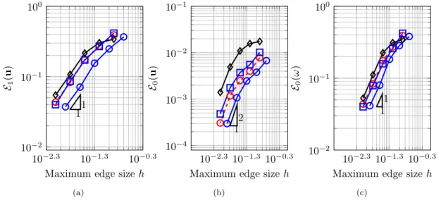
Employing postprocessing formulas and adequate polynomial projections we compute from the discrete stream- function further fields of interest, such as: the velocity and vorticity. Moreover, for these postprocessed variables we establish error estimates. Finally, we report practical numerical experiments on different families of polygonal meshes.

Key words: nonconforming virtual element, ocean circulation model, stream-function, error estimates, polygonal meshes, velocity-vorticity recovery.

Mathematics subject classifications (2000): 35Q35, 65N12, 65N15, 65N30

1 Introduction

The Stommel-Munk model in stream-function form is a linear fourth-order partial differential equation given by:

M∆²ψ−S∆ψ−∂xψ=f in Ω, (1.1)

with the boundary conditions:

ψ=∂_nψ= 0 on∂Ω, (1.2)

where Ω⊂R²is a simply connected domain with polygonal boundary∂Ω,∂_ndenotes the normal derivative,ψis the stream-function of the horizontal velocity fielduandf is the wind forcing term. In the model, the parameters M andS are the non-dimensional scale Munk and Stommel numbers, respectively, which are defined by:

M = A

βL³ and S = γ βL,

whereAis the eddy viscosity parametrization,Lis the characteristic length scale,β is the coefficient multiplying they-coordinate in theβ-plane approximation andγis the coefficient of the linear drag (or the Rayleigh friction), as might be generated by a bottom Ekman layer (for further details, see for instance [43,36,19,25]).

The Stommel-Munk model can be seen as a simplification of the Quasi-Geostrophic equations of the ocean (QGE) [25,28,27], both models are characterized by the presence of the biharmonic operator ∆²ψ, the rotational term ∂xψ, the source term f and they have the same boundary conditions (1.2), but the difference between these models lies in the presence of the nonlinear Jacobian operator in the QGE, whereas the linear Stommel- Munk model instead contains the Laplacian operator ∆ψ. Despite the simplifications, the Stommel-Munk model turns out to be adequate to understand the large scale wind-driven ocean circulation at mid-latitudes due to the model preserves principal features of these currents (the wind forcing and the effects of rotation). The above fact converts the Stommel-Munk model in a standard problem in the geophysical fluid dynamics literature (see

∗GIMNAP, Departamento de Matem´atica, Universidad del B´ıo-B´ıo, Concepci´on, Chile and Department of Mechanical Engineering, Indian Institute of Technology Madras, Chennai 600036, India. E-mail: [email protected]

†GIMNAP, Departamento de Matem´atica, Universidad del B´ıo-B´ıo, Concepci´on, Chile and CI²MA, Universidad de Concepci´on, Concepci´on, Chile. E-mail: [email protected]

‡GIMNAP, Departamento de Matem´atica, Universidad del B´ıo-B´ıo, Concepci´on, Chile. E-mail:

[email protected]

for instance [43,41, 34]), for which different finite element discretizations have been studied, for instance, using the stream function-vorticity formulation (see [36,24, 19]) and stream-function form. In particular, for the last formulation in [29] a B-spline based finite element discretization is introduced and error analysis for this scheme is developed in [42]. In [28] a discrete variational formulation based in C⁰-discontinuous Galerkin method is provided and error estimate for the scheme is performed. In the present contribution, we develop and analyze a nonconforming Morley-type virtual element scheme to approximate the Stommel-Munk model formulated in terms of the stream-function. This formulation have outstanding characteristics, such as: there is only one scalar unknown in the system, the streamlines is one of the most useful tools in flow visualization. Moreover, in this work we propose to obtain two variables of great interest in oceanic fluid dynamics: the velocity and vorticity fields, from the discrete stream-function by using postprocessing formulas.

The development of adequate numerical schemes for discretizing PDEs on general polytopal meshes have undergone an intensive research in the past years. Different approaches have been proposed (see for instance [8]

and the references therein) and among them we can find the Virtual Element Method (VEM), which since its introduction in the pioneering work [7] it has enjoyed a broad success in numerical modeling of scientific and engineering applications due to its elegant construction and promising results. A wide variety of problems have been addressed using the conforming VEM approach; see for instance [4,3,17,21,39], where second- and fourth- order problems have been analyzed. Moreover, in fluid mechanic the models studied, include: Stokes, Brinkman, Navier-Stokes flows and QGE; see for instance [15, 9, 11, 37, 10, 1, 38], where primal and mixed formulations have been considered.

On the other hand, the nonconforming VEM approach, also has presented a growing interest recently. Different schemes for several problems have been developed, for instance, second-order elliptic and fluid mechanic problems have been studied in [6,16,31,32,33,48,49]. Moreover, for fourth-order equations in [45] aH²-nonconforming VEM for plate bending problems is analyzed, which the numerical solution turns to beC⁰-continuous. Subse- quently, in [5] a fully nonconforming VEM for biharmonic problems is developed. In this space the approximated solution does not require the global C⁰-regularity. Besides, in [47] the authors, presented a VEM also for plate bending problems using the same degrees of freedom considered in [5]. However, the construction of the local virtual space have a different approach. The above fully nonconforming VEMs, in the lowest-order case (k= 2) can be seen as the extension of the Morley finite element [40] to polygonal meshes. For further nonconforming VEM involving fourth-order problems, see the references [18,26,46, 30, 44,23].

In the present work, we propose and analyze a nonconforming Morley-type virtual element discretization for the Stommel-Munk model (cf. (1.1)-(1.2)) with applications in large scale wind-driven oceanic circulation. We consider an enhanced nonconforming virtual space based on the approach presented in [30] (see also [5, 47] and [3]) to approximate the stream-function variable. This virtual element is characterized by not requiring any globalC⁰-regularity for the discrete solution and can be taken as a generalization of the classical Morley element to general polygonal meshes. Employing suitable projections operators, which are computable using only the degrees of freedom we construct the respective discrete bilinear forms and discrete load term. Then, we write a discrete virtual formulation and we prove its well-posedness by using the Lax-Milgram Theorem. We introduce an enriching operator from the enhanced nonconforming virtual space into its H²-conforming counterpart (see [4]). For the enhancedH²-conforming virtual space we recall its construction and we derive inverse inequalities and an equivalence between L²- and `²-norms, which are key tools to establish some approximation properties involving the enriching operator, the bilinear form associated to the inner productH² and the consistency error.

Then, with the help of these results we prove optimal error estimates for the stream-function in brokenH²-,H¹- and L²-norms under the minimal regularity of the weak solution (cf. Theorem 2.2). Moreover, we propose to compute further variables of interest, such as: the velocity field and the fluid vorticity by a simple postprocess of the discrete VEM stream-function and using suitable projections, which are computable from the degrees of freedom. Finally, we point out that, the present contribution is a good stepping stones for the nonlinear one- and two-layers QGE (see [25,38,27,35]).

The remaining part of the manuscript is organized as follows: in Subsection1.1we introduce some notations that will be used throughout the paper. In Section 2 we write a weak formulation for the system (1.1)-(1.2).

In Section3 we introduce the fully nonconforming virtual element scheme of the weak formulation. In Section 4 we present some preliminary results including the construction of an enriching operator from the enhanced nonconforming virtual space into itsH²-conforming counterpart. Besides, we derive useful tools to establish the optimal error estimate in brokenH²-norm up to the regularity of the weak solution. Moreover, we obtain optimal error estimates in broken H¹- and L²-norms by using duality arguments and under the same regularity of the continuous solution. In Section 5 we compute the velocity field and fluid vorticity by a simple postprocess of the discrete VEM stream-function. Finally, in Section 6 we report some numerical experiments exhibiting the behaviour of our virtual scheme and confirming the our theoretical results.

The major contribution of the article can be summarized as follows:

• In this article, we extend the fully nonconforming virtual element approach [5,47] (see also [30]) to solve

the fourth order Stommel-Munk model on polygonal meshes and we establish error estimates in broken H²-, H¹- and L²-norms under the minimal regularity by introducing enriching operator as mentioned in Section 4.2. Furthermore, the error estimations in brokenL²- andH¹-norms have been derived assuming the source termf belongs to L²(Ω). Moreover, we have proposed novel strategies to compute the velocity and vorticity fields as a postprocess of the discrete stream-function using suitable polynomial projections.

1.1 Notations

From now on, we will follow the usual notation for Sobolev spaces, seminorms and norms [2]. We will denote a simply connected polygonal Lipschitz bounded domain ofR²by Ω andn= (ni)_1≤i≤2 is the outward unit normal vector to the boundary∂Ω, while the vectort= (ti)i=1,2 is the unit tangent to∂Ω oriented such thatt1=−n2, t2 = n1. In addition, for any vector field v = (vi)i=1,2 and any scalar function ϕ, we define the differential operators:

rotv:=∂1v2−∂2v1, ∇ϕ:=

∂1ϕ

∂2ϕ

and curlϕ:=

∂2ϕ

−∂1ϕ

.

Moreover, D²ϕ:= (∂ijϕ)i,j=1,2denotes the matrix Hessian ofϕ.

In addition, in this work,candC, with or without superscripts and subscripts, tildes or hats, will represent a strictly positive constant independent of the mesh parameterh, whose value can change in different occurrences.

2 The continuous formulation

Let V := {ϕ ∈ H²(Ω) : ϕ = ∂nϕ = 0 on ∂Ω}. Then, we have that a variational formulation of problem (1.1)-(1.2) is given as follows: seekψ∈ V, such that

A(ψ, φ) =F(φ) ∀φ∈ V, (2.1)

where

A(ϕ, φ) :=MAD(ϕ, φ) +SA∇(ϕ, φ)−Askew(ϕ, φ) ∀ϕ, φ∈ V, (2.2) and the formsAD(·,·), A∇(·,·), Askew(·,·) andF(·) are defined by:

AD:V × V −→R, AD(ϕ, φ) :=

Z

Ω

D²ϕ: D²φ ∀ϕ, φ∈ V, (2.3)

A_∇:V × V −→R, A_∇(ϕ, φ) :=

Z

Ω

∇ϕ· ∇φ ∀ϕ, φ∈ V, (2.4)

Askew:V × V −→R, Askew(ϕ, φ) :=1 2

Z

Ω

∂xϕφ−1 2

Z

Ω

∂xφ ϕ ∀ϕ, φ∈ V, (2.5) F :V −→R, F(φ) :=

Z

Ω

f φ ∀φ∈ V. (2.6)

Remark 2.1 We recall that the classical variational formulation of problem (1.1)-(1.2)is given by: findψ∈ V, such that

MAD(ψ, φ) +SA∇(ψ, φ)−A0(ψ, φ) =F(φ) ∀φ∈ V, where

A₀(ψ, φ) :=

Z

Ω

∂_xψ φ.

We observe that the bilinear formA0(·,·)is equal to the skew-symmetric formAskew(·,·)defined in(2.5). However, their discrete versions will lead to different bilinear forms, in general. Therefore, we point out that, our virtual method will be based on the weak formulation (2.1), keeping the skew-symmetric property for the bilinear form A_skew(·,·), which allows making the analysis of the scheme in a straightforward way.

We endow the space V with the normkϕkV := (AD(ϕ, ϕ))^1/2 ∀ϕ∈ V, then the forms defined in (2.3)-(2.6) are continuous. More precisely, in the following lemma we summarize some properties for the forms defined in (2.2) and (2.6), which will be used to establish the well-posedness of problem (2.1).

Lemma 2.1 For all ϕ, φ∈ V, there exists a positive constantsCA, such that the formsA(·,·) andF(·), defined in (2.2) and (2.6), respectively, satisfy the following properties:

• |A(ϕ, φ)| ≤ CAkϕk_Vkφk_V; • A(φ, φ)≥Mkφk²_V; • |F(φ)| ≤ kFk_−2,Ωkφk_V. Theorem 2.1 There exists a unique ψ ∈ V solution to problem (2.1), which satisfies the following continuous dependence on the data

kψkV≤CkFk−2,Ω, whereC is a positive constant.

Proof. It is an immediate consequence of Lemma2.1and the Lax-Milgram Theorem.

Now, we will state an additional regularity result for the solution of problem (2.1).

Theorem 2.2 Let ψ∈ V be the unique solution of problem (2.1). If F ∈H⁻¹(Ω), then there exist s∈(1/2,1]

andCreg>0 such that ψ∈H^2+s(Ω)and

kψk2+s,Ω≤C_regkFk−1,Ω.

Proof. The proof follows from the classical regularity result for the biharmonic problem with homogeneous

Dirichlet boundary conditions (see for instance [12]).

3 Nonconforming virtual element discretization

In this section we will introduce a Morley-type VEM for the numerical approximation of problem (2.1) on general polygonal meshes, which is based on the fully nonconforming virtual element approach [5, 47, 30]. First, we introduce some notations to present the local and global nonconforming virtual space. Successively, we introduce some projectors on polynomial spaces to construct the discrete bilinear forms and discrete functional. Finally, we write the discrete problem and we establish its well-posedness by using the Lax-Milgram Theorem.

3.1 Notations and basic setting

Henceforth, we will denote by K a general polygon, by h_K and ∂K its diameter and boundary, respectively.

Moreover, we will denote byN_K the number of vertices ofK. Let{Th}_h>0be a sequence of decompositions of Ω into general non-overlapping simple polygonsK, whereh:= max_K∈Thh_K. We will denote the set of the edges in ThbyEh, we decompose this set asEh:=Eh^int∪E_h^bdry, whereEh^intandE_h^bdry are the set of interior and boundary edges, respectively. Analogously, we will denote by Vh :=Vh^int∪Vh^bdry the set of the all vertices inTh, where Vh^int and Vh^bdry are the the set of interior and boundary vertices, respectively.

Additionally, for eachK∈Th, we denote byn_K its unit outward normal vector and byt_K its tangential vector along the boundary∂K. Besides, we will use the notation n_eand t_efor a unit normal and tangential vector of an edgee∈Eh, respectively.

For any subsetD ⊂R² and each integer `≥0 we denote byP`(D) the space of polynomials of degree up to` defined onD. Moreover, we define the piecewise `-order polynomial space by:

P`(Th) :={q∈L<sup>2</sup>(Ω) :q|K ∈P`(K) ∀K∈Th}.

Next, for any integer numbert >0, we introduce the following broken Sobolev space H^t(Th) :={φ∈L²(Ω) :φ|K∈H^t(K) ∀K∈Th} endowed with the following broken seminorm

|φ|_t,h:= X

K∈Th

|φ|²_t,K^1/2

. (3.1)

Now, we will define the jump operator denoted by [[·]], as follow: for each functionφ∈H²(Th) and for an internal edge e ∈ Eh^int, we define [[φ]] := φ⁺−φ⁻, where φ^± denotes the trace of φ|_K±, withe ⊆ ∂K⁺∩∂K⁻. For a boundary edgee∈E_h^bdry, the operator jump is define as: [[φ]] :=φ|_e.

We introduce a subspace ofH²(Th) with certain continuity, given by:

H^2,NC(Th) :=

(

φh∈H²(Th) :φhcontinuous at internal vertices,

φ_h(v_i) = 0 ∀v_i∈V_h^bdry, Z

e

[[∂_neφ_h]] = 0 ∀e∈Eh

) .

(3.2)

For the theoretical analysis, we suppose thatTh satisfies the following assumptions: there exists a real number ρ >0 such that, everyK∈Th, we have

A₁: K is star-shaped with respect to every point of a ball of radius≥ρh_K;

A2: the ratio between the shortest edge and the diameterhK ofK is larger thanρ.

We decompose the continuous forms defined in (2.2)-(2.5) as follows:

AD(ϕ, φ) = X

K∈Th

A^K_D(ϕ, φ) := X

K∈Th

Z

K

D²ϕ: D²φ ∀ϕ, φ∈ V,

A_∇(ϕ, φ) = X

K∈Th

A^K_∇(ϕ, φ) := X

K∈Th

Z

K

∇ϕ· ∇φ ∀ϕ, φ∈ V,

A_skew(ϕ, φ) = X

K∈Th

A^K_skew(ϕ, φ) := X

K∈Th

1 2

Z

K

∂_xϕ φ−1 2

Z

K

∂_xφ ϕ ∀ϕ, φ∈ V.

Also, we split

A(ϕ, φ) = X

K∈Th

A^K(ϕ, φ) := X

K∈Th

(_MA^K_D(ϕ, φ) +_SA^K_∇(ϕ, φ)−A^K_skew(ϕ, φ)) ∀ϕ, φ∈ V.

3.2 Local and global nonconforming virtual element spaces

For every polygonK∈Th, we introduce the following preliminary local virtual space (for further details see [30, Section 3.4] and [5,47,3]):

Veh(K) :=

φh∈H²(K) : ∆²φh∈P2(K), φh|e∈P2(e), ∆φh|e∈P0(e) ∀e⊆∂K .

Next, for a given φh ∈ Veh(K), we introduce the following set of linear operators (which will be degrees of freedom after of the enhancement technique):

• D1: the values ofφh(vi) for all vertexvi of the polygon K;

• D2: the moments

Z

e

∂n_eφh ∀edgee⊆∂K.

For each polygonK, we define the following projector

Π^D_K:Veh(K)−→P2(K)⊆Veh(K), φ_h7−→Π^D_Kφ_h,

where Π^D_Kφh is the solution of the local problems:

A^K_D(Π^D_Kφh, q) =A^K_D(φh, q) ∀q∈P2(K), Π\^D_Kφ_h=cφ_h

Z

∂K

∇Π^D_Kφ_h= Z

∂K

∇φ_h,

and the operatorc(·) is defined as follows:

ϕch:= 1 N_K

N_K

X

i=1

ϕh(vi), (3.3)

andvi, 1≤i≤NK are the vertices ofK.

Moreover, as stated by the following lemma, the polynomial projection Π^D_K is computable using the sets D₁ andD₂ (for more details see [47, 30]).

Lemma 3.1 The operator Π^D_K :Veh(K)−→P2(K)is explicitly computable for every φ_h∈Veh(K), using only the information of the linear operators D₁ andD₂.

Now, for eachK∈Th we introduce the enhanced fully nonconforming virtual space:

V_h(K) :=

(

φ_h∈Ve_h(K) : Z

e

(φ_h−Π^D_Kφ_h) = 0 ∀e⊆∂K, Z

K

p(φ_h−Π^D_Kφ_h) = 0 ∀p∈P2(K) )

. (3.4)

The following result summarize the main properties of the local virtual spaceVh(K). The proof can be obtained following the arguments in [5,47,3,30].

Proposition 3.1 For each polygon K, the space Vh(K)defined in (3.4)satisfies the following properties:

• P2(K)⊆ V_h(K).

• The sets of linear operators D₁ andD₂ constitutes a set of degrees of freedom forV_h(K).

• The operator Π^D_K :Vh(K)−→P2(K)is computable using the degrees of freedom D1 andD2.

Now, for every decomposition Th of Ω into polygons K, we introduce the fully nonconforming global virtual space to the numerical approximation of problem (2.1) as follows:

Vh:=

φ_h∈H^2,NC(Th) :φ_h|K ∈ Vh(K) ∀K∈Th , (3.5) where the spaceH^2,NC(Th) is defined in (3.2).

It is observed thatVh⊆H^2,NC(Th) butVh*V. Furthermore, we have that the nonconforming virtual element does not require theC⁰-continuity over Ω.

3.3 Polynomial projection operators

In this subsection, we introduce further polynomial projections, which will be useful to build the respective discrete forms.

First, for allm∈N∪ {0}, we consider the usualL²(K)-projection onto the polynomial spacePm(K): for each φ∈L²(K), the function Π^m_Kφ∈P^m(K) is defined as the unique function satisfying

(q, φ−Π^m_Kφ)_0,K = 0 ∀q∈Pm(K). (3.6)

Lemma 3.2 Let Π²_K be the operator defined in (3.6), withm= 2. Then, for eachφ_h∈ Vh(K) we have that the polynomial functionsΠ²_Kφ_h andΠ²_K(∂_xφ_h)are computable using only the information of the degrees freedom D₁ andD₂.

Proof. Letφ_h ∈ Vh(K). Then the function Π²_Kφ_h is easily obtained from the definition of the space Vh(K) (cf.

(3.4)). On the other hand, using integration by parts and the definition of Π²_Kφ_h, for allq∈P2(K), we have Z

K

∂_xφ_hq=− Z

K

φ_h∂_xq + Z

∂K

φ_hqn^x_K =− Z

K

(Π²_Kφ_h)∂_xq + Z

∂K

φ_hqn^x_K,

where n^x_K is the first component of normal vectorn_K. We notice that the first term on the right hand side of the above equality depends only on Π²_Kφ_h, hence computable using the degrees of freedom (see Proposition3.1).

The boundary integral is computable usingD₁and the moments of Π^D_Kφ_h on the each edgee⊆∂K (cf. (3.4)).

Next, for each polygonK, we define the projector Π^∇_K :Vh(K)−→P2(K)⊆ Vh(K), as the solution of the local problems:

A^K_∇(Π^∇_Kφ_h, q) =A^K_∇(φ_h, q) ∀q∈P2(K), (3.7a)

Π\^∇_Kφ_h=φc_h, (3.7b)

and the operatorc(·) is defined in (3.3).

The following result establishes that the polynomial projection Π^∇_K is computable from the sets D1 and D2. The result follows the same arguments used in the proof of Lemma3.2.

Lemma 3.3 The operator Π^∇_K :Vh(K)−→P2(K)is explicitly computable for every φh∈ Vh(K), using only the information of the linear operators D1 andD2.

3.4 Construction of the discrete forms

In the present section, we will build the discrete version of the continuous local forms defined in (2.3)-(2.6) by using the operators introduced in the above subsection.

First, letS_D^K(·,·) andS_∇^K(·,·) be any symmetric positive definite bilinear forms to be chosen as to satisfy:

c₀A^K_D(φ_h, φ_h)≤ S_D^K(φ_h, φ_h)≤c₁A^K_D(φ_h, φ_h) ∀φh∈ Vh(K), with Π^D_Kφ_h= 0,

c₂A^K_∇(φ_h, φ_h)≤ S_∇^K(φ_h, φ_h)≤c₃A^K_∇(φ_h, φ_h) ∀φ_h∈ V_h(K), with Π^∇_Kφ_h= 0, (3.8) withc0, c1, c2andc3 positive constants independent ofhandK. A classical choice for the bilinear formsS_D^K(·,·) andS_∇^K(·,·) satisfying (3.8) is given by the Euclidean scalar product associated to the degrees of freedom scaled appropriately (see [6,5,47]). More precisely, we choose the following representation:

S_D^K(ϕh, φh) :=h⁻²_K

N_dof^K

X

i=1

dofi(ϕ)dofi(φ) and S_∇^K(ϕh, φh) :=

N_dof^K

X

i=1

dofi(ϕ)dofi(φ),

for allϕ_h, φ_h∈ V_h(K), whereN_dof^K denote the number of degrees freedom ofV_k^h(K) and dof_iis the operator that to each smooth enough functionφassociates theith local degree of freedom dof_i(φ), with 1≤i≤N_dof^K .

Thus, we define the following global formA^h:Vh× Vh−→R, given by:

A^h(ϕh, φh) = X

K∈Th

A^h,K(ϕh, φh) = X

K∈Th

(MA^h,K_D (ϕh, φh) +MA^h,K_∇ (ϕh, φh)−A^h,K_skew(ϕh, φh)), (3.9)

where the discrete local bilinear forms, A^h,K_D : Vh(K)× Vh(K) −→ R, A^h,K_∇ : Vh(K)× Vh(K) −→ R and A^h,K_skew :Vh(K)× Vh(K)−→R, approximating the continuous bilinear forms A^K_D(·,·), A^K_∇(·,·) and A^K_skew(·,·) are given by

A^h,K_D (ϕh, φh) :=A^K_D Π^D_Kϕh,Π^D_Kφh

+S_D^K (I−Π^D_K)ϕh,(I−Π^D_K)φh

, (3.10)

A^h,K_∇ (ϕh, φh) :=A^K_∇ Π^∇_Kϕh,Π^∇_Kφh

+S_∇^K (I−Π^∇_K)ϕh,(I−Π^∇_K)φh

, (3.11)

A^h,K_skew(ϕ_h, φ_h) := 1 2 Z

K

Π²_K(∂_xϕ_h) Π²_Kφ_h−1 2

Z

K

Π²_K(∂_xφ_h) Π²_Kϕ_h. (3.12) The following result establishes the usual consistency and stability properties for the discrete local forms.

Proposition 3.2 The local bilinear forms A^K_D(·,·),A^K_∇(·,·),A^K(·,·),A^h,K_D (·,·),A^h,K_∇ (·,·)andA^h,K(·,·)on each elementK satisfy

• Consistency: for all h >0and for all K∈Th, we have that

A^h,K(q, φh) =A^K(q, φh) ∀q∈P2(K), ∀φh∈ Vh(K), (3.13)

• Stability and boundedness: There exist positive constants α_i, i= 1, . . . ,4independent of K, such that:

α1A^K_D(φh, φh)≤A^h,K_D (φh, φh)≤α2A^K_D(φh, φh) ∀φh∈ Vh(K), (3.14) α₃A^K_∇(φ_h, φ_h)≤A^h,K_∇ (φ_h, φ_h)≤α₄A^K_∇(φ_h, φ_h) ∀φh∈ Vh(K). (3.15) Proof. The proof follows standard arguments in the VEM literature (see [7, 5,47]).

Finally, we consider the following approximation of the functional defined in (2.6):

F^h(φh) := X

K∈Th

F^h,K(φh) ∀φh∈ Vh, (3.16)

where, for the local functionalF^h,K(·), is defined by:

F^h,K(φh) :=

Z

K

Π²_Kf φh≡ Z

K

fΠ²_Kφh ∀φh∈ Vh(K).

For the continuous bilinear formsA_?(·,·), with?∈ {D,∇,skew}, we adopt the following notation:

A_?(ϕ_h, φ_h) := X

K∈Th

A^K_?(ϕ_h, φ_h) ∀ϕh, φ_h∈ Vh. (3.17) We also adopt the same notation by the bilinear formA(·,·) and the functionalF(·).

3.5 Discrete problem and its well-posedness

In this subsection, we present the discrete virtual element formulation and we establish its well-posedness by using the Lax-Milgram Theorem.

The fully nonconforming virtual element problem reads as: seekψ_h∈ V_h, such that

A^h(ψ_h, φ_h) =F^h(φ_h) ∀φ_h∈ V_h, (3.18) where A^h(·,·) is the discrete bilinear forms defined in (3.9) and F^h(·) is the discrete functional introduced in (3.16).

The following lemma establishes properties for the application| · |2,h defined in (3.1), witht= 2.

Lemma 3.4 For all φh∈ Vh, the following inequality holds:

kφhk0,Ω+|φh|1,h≤C|φh|2,h,

whereC is a positive constant, independent of h. Moreover, we have that | · |2,h is a norm on the spaceVh.

Proof. The proof is established in [47, Lemma 5.1].

The following result establishes some properties for the discrete forms defined in the last subsection, which will be used to conclude the well-posedness of the discrete problem (3.18). The proof follows from the definition of the respective forms.

Lemma 3.5 For all ϕh, φh ∈ Vh, there exist positive constants C_Ah,α, Ce _Fh, independent of h, such that the forms defined in (3.12),(3.9)and (3.16)satisfy the following properties:

|A^h(ϕ_h, φ_h)| ≤C_Ah|ϕh|2,h|φh|2,h, A^h(φ_h, φ_h)≥α|φe h|²_2,h, (3.19) A^h,K_skew(φ_h, φ_h) = 0, |F^h(φ_h)| ≤C_Fhkfk0,Ω|φh|2,h. (3.20) We have the following result of existence and uniqueness.

Theorem 3.1 The discrete problem (3.18) admits a unique solution ψ_h ∈ V_h, which satisfies the following continuous dependence on the data

|ψh|2,h≤Ckfk0,Ω, where the positive constantC is independent ofh.

Proof. It is an immediate consequence of Lemma3.5and the Lax-Milgram Theorem.

4 Convergence analysis

In this section we will establish error estimates for the nonconforming VEM presented in Section3.5. First, we present some preliminary results useful for the analysis. Successively, we introduce anenriching operatorE_hfrom the nonconforming space V_h into its conforming counterpart. Then, we derive some approximation properties involving this operator and the bilinear form A_D(·,·) (cf. (2.3)). By using the above tools we establish an error estimate in broken H²-norm under minimal regularity condition on the stream-function ψ (cf. Theorem 2.2).

Finally, by using duality arguments we derive error estimates in broken H¹- and L²-norms under the same regularity of the weak solution and assuming the source termf belongs toL²(Ω).

4.1 Preliminary results

We start recalling an important approximation result for polynomials on star-shaped domains (see, for instance [13,30]).

Proposition 4.1 Assume that A1 is satisfied. Then, for every φ∈ H^2+t(K), with t ∈ [0,1], there exist φπ ∈ P2(K) andC >0, independent ofh, such that

kφ−φπk`,K≤Ch<sup>2+t−`</sup>_K |φ|2+t,K, `= 0,1,2.

We have the following approximation result in the virtual spaceVh (see [5, 47,30]).

Proposition 4.2 Assume that A1−A2 are satisfied. Then, for each φ ∈H^2+t(Ω), with t ∈[0,1], there exist φI ∈ Vh andC >0, independent of h, such that

kφ−φIk`,K≤Ch<sup>2+t−`</sup>_K |φ|2+t,K, `= 0,1,2.

We have the following estimation involving the continuous and discrete functionals.

Proposition 4.3 Letf ∈L²(Ω)and letF(·)andF^h(·)be the functionals defined in(2.6)and(3.16), respectively.

Then under assumptionA1, we have the following estimate:

kF−F^hk_V⁰

h := sup

φh∈Vh

φ_h6= 0

|F(φh)−F^h(φh)|

|φh|2,h

≤Ch²kfk0,Ω.

Proof. The proof follows from the definition of the functionals F(·) and F^h(·), together with approximation

property of the projector Π²_K.

We finish this subsection presenting some technical lemmas, which will be useful in the next sections. Proof of this results can be obtained following arguments of [13,20,26].

Lemma 4.1 There existsC >e 0, independent of hK, such that

kqk0,K≤Che ⁻ⁱ_Kkqk_−i,K ∀q∈P<sup>`</sup>(K), `≥0, i= 1,2.

Lemma 4.2 If the assumption A1 is satisfied, for eachε >0, there exist positive constantsC, Cε, independent of h_K, such that

kϕk0,∂K≤C1(εh^1/2_K |ϕ|1,K+Cεh^−1/2_K kϕk0,K) ∀ϕ∈H¹(K),

|ϕ|1,K≤C2(εhK|ϕ|2,K+Cεh⁻¹_K kϕk0,K) ∀ϕ∈H²(K).

Lemma 4.3 The projectionΠe⁰_e:L²(K)−→P0(e)defined by the following average Πe⁰_eϕ:= 1 he

Z

e

ϕds, satisfies

kϕ−Πe⁰_eϕk0,e≤Ch^1/2_K |ϕ|1,K ∀ϕ∈H¹(K).

4.2 Enriching operator

In this subsection, we will focus on proposing and analyzing an enriching operatorEhfrom the enhanced noncon- forming spaceVhinto its H²-conforming counterpart. Following the ideas of [26], we can construct an enriching operatorEh:Vh−→ V_h^C, whereV_h^Cis the enhancedH²-conforming virtual element space considered in [4]. The construction is based on the degrees of freedom ofV_h^C.

For the sake of completeness, we will recall the construction of the virtual enhancedH²-conforming space of lowest order and the enriching operatorE_h.

Conforming virtual local space. For every polygon K ∈Th, we introduce the following preliminary finite dimensional space [4]:

Ve_h^C(K) :=

φ_h∈H²(K) : ∆²φ_h∈P2(K), φ_h|∂K ∈C⁰(∂K), φ_h|e∈P3(e)∀e⊆∂K,

∇φh|∂K ∈[C⁰(∂K)]², ∂n_eφh|e∈P1(e)∀e⊆∂K ,

Next, for a given φh ∈ Ve_h^C(K), we introduce two sets D1^v and D2^∇ of linear operators from the local virtual spaceVe_h^C(K) intoR:

• D1^v: the values ofφ_h(v) for all vertexv∈∂K,

• D2^∇: the values ofh_v∇φh(v) for all vertexv∈∂K,

where hv is a characteristic length attached to each vertex v, for instance to the maximum diameter of the elements withvas a vertex. Now, we consider the operator Π^D,C_K :Ve_h^C(K)−→P2(K)⊆Ve_h^C(K) associated to the conforming approach, which is computable using the setsD1^v andD2^∇(for more details see [4, Lemma 2.1]).

Next, for eachK∈Th, we introduce the conforming local enhanced virtual space as follows:

V_h^C(K) :=n

φh∈Ve_h^C(K) : (φh−Π^D,C_K φh, q)0,K = 0 ∀q∈P2(K)o

. (4.1)

In this space the setsD1^v andD2^∇constitutes a set of degrees of freedom.

Conforming virtual global space. For every decompositionThof Ω into polygonsK, we define the conform- ing virtual spacesV_h^C:

V_h^C:=

φh∈ V: φh|K∈ V_h^C(K) ∀K∈Th . (4.2)

For a vertexv∈Vh, we denote by ω(v) the union of all elements inTh, sharing the vertexvand byN(v) the number of elements ofω(v). For anyϕh∈ Vh, we introduce the piecewiseL²-projection Π², as follows:

Π²ϕh|K = Π²_K(ϕh|K),

where Π²_K is theL²-projection fromVh(K) ontoP2(K) (cf. Lemma 3.2) and Vh(K) is the local nonconforming virtual space defined in (3.4). For each functionϕh∈ Vh, the functionEhϕh∈ V_h^Cin the conforming counterpart will be constructed as follows:

Eh(ϕh)(x) =

N_dof^C

X

i=1

Di(Eh(ϕh))χi(x),

where the functions {χi}^N_i=1^dofC are the set of shape basis functions associated to space V_h^C andN_dof^C := dim(V_h^C).

More precisely, the values of degrees of freedom for the enriching operator are determined as follows:

1. For the values at interior vertices v∈V_h^int, we consider:

D1^v(Ehϕh) := 1 N(v)

X

K∈ω(v)e

Π²ϕh|

Ke(v).

2. For the gradient values at interior verticesv∈Vh^int, we consider:

D1^∇(Ehϕh) := 1 N(v)

X

K∈ω(v)e

hv∇(Π²ϕh|

Ke)(v).

We will denote byχ(·) :={χ_v,χ_∇} the degrees of freedom vector corresponding to theH²-conforming virtual element spaceV_h^C(K), withχ_v collecting the degrees of freedom inD1^v andχ_∇ the degrees of freedom inD2^∇.

In what follows, we will derive some approximation properties for the operator Eh. To do that, first we will establish two technical tools: inverse inequalities for the enhanced H²-conforming virtual spaceV_h^C(K) defined in (4.2) and a norm equivalence between the degrees of freedom vectorχandL²-norm.

In order to establish the results mentioned above, first we will consider three preliminary lemmas. We start with anH²-orthogonal decomposition.

Lemma 4.4 Any function φ∈H²(K)admits the decompositionφ=φ₁+φ₂,where 1. φ1∈H²(K),φ1|∂K=φ|∂K,∂n_Kφ1=∂n_Kφand∆²φ1= 0 in K.

2. φ2∈H₀²(K),∆²φ2= ∆²φ in K.

Moreover, this decomposition isH²-orthogonal in the sense that

|φ|²_2,K=|φ1|²_2,K+|φ2|²_2,K.

Proof. Letφ∈H²(K), then we can choose φ₂ as theH²-projection of φtoH₀²(K), i.e., we define φ₂ ∈H₀²(K) as the unique solution of the following local problem:

Z

K

D²φ2: D²ϕ= Z

K

D²φ: D²ϕ ∀ϕ∈H₀²(K).

Thus, we define φ₁ := (φ−φ₂) ∈H²(K). We notice that by construction the functions φ₁ and φ₂ satisfy the

properties of lemma.

For the functionsφ₁andφ₂of the above decomposition, we will derive useful inequalities to establish an inverse estimate in theH²-conforming virtual space V_h^C(K). For the biharmonic part, we have the next inequality.

Lemma 4.5 For any ε >0, there exist positive constants C, Cε, independent of hK, such that

|φ1|2,K≤C(ε|φ|2,K+Cεh⁻²_K kφk0,K).

Proof. Letφ∈ V_h^C(K) andφ1∈H²(K) such that Lemma4.4holds true. Then, we define the space Sφ₁(K) :=

ϕ∈H²(K) :ϕ|∂K =φ1|∂K, ∂n_Kϕ=∂n_Kφ1 .

For eachϕ∈Sφ₁(K) we have thatϕ−φ1∈H₀²(K). Then, since ∆²φ1= 0 in K, applying integration by part we get

Z

K

D²φ₁: D²(ϕ−φ₁) = 0, which implies

|ϕ|²_2,K=|φ1|²_2,K+|ϕ−φ1|²_2,K. Therefore,

|φ1|2,K≤ |ϕ|2,K ∀ϕ∈Sφ1(K). (4.3) Now, for everyK∈Th, letTK be the sub-triangulation obtained by connecting each vertex ofKwith the center of the ball with respect to whichK is starred (cf. Assumption A₁). Then, on each triangle of TK we consider the reduced Hsieh-Clough-Tocher element (HCT) defined in [22]. Thus, forφ∈ V_h^C(K) we choose the interpolant I_Kφin the HCT element, for which it is fulfilled that

IKφ|∂K =φ|∂K=φ1|∂K and ∂n_K(IKφ) =∂n_Kφ=∂n_Kφ1. Hence,IKφ∈Sφ₁(K) and by the definition ofIKφ, we also have the following estimate

kI_Kφk_0,K≤C(h^1/2_K kI_Kφk_0,∂K+h^3/2_K k∂_nK(I_Kφ)k_0,∂K)

=C(h^1/2_K kφk_0,∂K+h^3/2_K k∂_nKφk_0,∂K).

(4.4) Then, takingϕ=I_Kφ∈S_φ1(K) in (4.3) and using the inverse inequality for polynomials (cf. Lemma 4.1) and estimate (4.4), we obtain

|φ1|2,K ≤ |IKφ|2,K≤Ch⁻²_K kIKφk0,K≤C(h^−3/2_K kφk0,∂K+h^−1/2_K k∂n_Kφk0,∂K). (4.5) Next, we will estimate the two terms on the right hand side of (4.5). Indeed, from Lemma4.2, for every ε >0, there existC, Cε>0, independent ofh, such that

h^−3/2_K kφk_0,∂K≤Ch^−3/2_K (εh^1/2_K |φ|_1,K+C_εh^−1/2_K kφk_0,K)≤C(ε|φ|_2,K+C_εh⁻²_K kφk_0,K). (4.6) Now, for the second term in (4.5) we notice that

k∇φk²_0,∂K= Z

∂K

∇φ· ∇φ=k∂nKφk²_0,∂K+k∂tKφk²_0,∂K ≤(k∂nKφk0,∂K+k∂tKφk0,∂K)². (4.7) From the above identity and Lemma4.2, for everyε >0, there exist C, Cε>0, independent ofh, such that

h^−1/2_K k∂n_Kφk0,∂K≤C(ε|φ|2,K+Cεh⁻²_K kφk0,K). (4.8) Then, the desired result follows inserting the estimates (4.6) and (4.8) in (4.5).

For the functionφ₂ of the decomposition in Lemma4.4, we have the following result.

Lemma 4.6 For any ε >0, there exists positive constants C, Cε, independent ofhK, such that

|φ2|2,K≤C(ε|φ|2,K+C_εh⁻²_K kφk0,K).

Proof. Let φ ∈ V_h^C(K) and φ2 ∈ H²(K) such that the Lemma 4.4 holds true. Then, since φ2 ∈ H₀²(K) and

∆²φ2 = ∆²φ∈ P2(K) in K, we use an integration by part, the Cauchy-Schwarz and inverse inequalities for polynomials (cf. Lemma4.1) to obtain

|φ₂|²_2,K= Z

K

φ₂∆²φ₂≤ k∆²φ₂k_0,Kkφ₂k_0,K≤Ch⁻²_K k∆²φ₂k_−2,Kkφ₂k_0,K≤Ch⁻²_K |φ₂|_2,Kkφ₂k_0,K. From the above estimate, Lemma4.4and the triangle inequality, we get

|φ2|2,K ≤Ch⁻²_K kφ2k0,K=Ch⁻²_K kφ−φ1k0,K ≤Ch⁻²_K kφk0,K+Ch⁻²_K kφ1k0,K. (4.9)

In what follows, we will establish estimates for the second term on the right hand side in (4.9). Applying the Poincar´e–Friedrichs inequality forH² functions, Cauchy-Schwarz inequality and using (4.7), we get

kφ1k0,K ≤C

h²_K|φ1|2,K+ Z

∂K

φ1

+hK

Z

∂K

∇φ1

≤C(h²_K|φ1|2,K+h^1/2_K kφ1k0,∂K+h^3/2_K (k∂n_Kφ1k0,∂K+k∂t_Kφ1k0,∂K)).

(4.10)

Now, we observe that φ1|e=φ|e ∈P3(e) ∀e⊆∂K. Then, by using standard inverse estimate for polynomials in one variable, we have

k∂t_Kφ1k0,∂K≤Ch⁻¹_K kφ1k0,∂K. Thus, inserting the above estimation in (4.10) we get

kφ1k0,K≤C(h²_K|φ1|2,K+h^1/2_K kφk0,∂K+h^3/2_K k∂nKφk0,∂K),

where we have used the fact that φ₁|∂K =φ|∂K and ∂_nKφ₁=∂_nKφ. Now, employing the above estimates and both inequalities of Lemma4.2we get

kφ1k0,K≤(h²_K|φ1|2,K+h^3/2_K k∂nKφk0,∂K+h^1/2_K kφk0,∂K)

≤C(h²_K|φ1|2,K+εh²_K|φ|2,K+Cεkφk0,K), which implies along with Lemma4.5that

h⁻²_K kφ1k0,K≤C(|φ1|2,K+ε|φ|2,K+Cεh⁻²_K kφk0,K)

≤C(ε|φ|_2,K+C_εh⁻²_K kφk_0,K). (4.11) From the estimates (4.9) and (4.11) for any ε >0, there exists positive constants C, Cε, independent ofhK, such that

|φ2|2,K ≤C(h⁻²_K kφk0,K+Ch⁻²_K kφ1k0,K)≤C(ε|φ|2,K+C_εh⁻²_K kφk0,K).

The proof is complete.

We have the following inverse inequalities for theH²-conforming spaceV_h^Cdefined in (4.1).

Lemma 4.7 For any φh∈ V_h^C(K), there exists a positive constantC, independent ofhK, such that

|φh|2,K≤Ch⁻²_K kφhk0,K and |φh|1,K ≤Ch⁻¹_K kφhk0,K. (4.12) Proof. Letφ_h ∈ V_h^C(K) and φ_h,1, φ_h,2 such that Lemma4.4holds true. Then, employing the triangle inequality together with Lemmas4.5and4.6, we have

|φ_h|_2,K≤ |φ_h,1|_2,K+|φ_h,2|_2,K≤C(ε|φ_h|_2,K+C_εh⁻²_K kφ_hk_0,K),

where C and C_ε are independent of h_K. Then, choosing εsmall enough and absorbing the term Cε|φ_h|_2,K on the left hand side of the above estimate we obtain the first inverse inequality in (4.12). The second inequality in (4.12) is an immediate consequence of the first estimate and Lemma4.2.

Now we will establish a norm equivalence between the degrees of freedom vectorχand theL²-norm.

Lemma 4.8 For any φh∈ V_h^C(K), there exist positive constantsC1 andC2, independent ofhK, such that C₁h_Kkχ(φ_h)k_{`</sub>2 ≤ kφ<sub>h</sub>k<sub>0,K</sub> ≤C<sub>2</sub>h<sub>K</sub>kχ(φ<sub>h</sub>)k<sub>`}2.

Proof. Letφh ∈ V_h^C(K). Then, for the lower bound, we have theφh|∂K and∂n_Kφh are polynomial functions on each edge of∂K. Therefore, using standard scaling argument we have

hKkχ(φh)k_`2≤C(h^1/2_K kφhk0,∂K+h^3/2_K k∂n_Kφhk0,∂K).

Now, following similar arguments to those used in Lemmas4.5and4.6, we have hKkχ(φh)k_`2 ≤C(h²_K|φh|2,K+kφhk0,K).

Therefore, applying the first the inverse inequality in (4.12) we get h_Kkχ(φ_h)k_`2 ≤Ckφ_hk_0,K.

To obtain the upper bound we proceed as in [26, Lemma 3.6].

Employing the above lemmas, we can establish the following approximation properties for the enriching operator Eh, which will play a important role to obtain a priori error estimate of our scheme under minimal regularity condition on the exact solution.

Lemma 4.9 For all ϕh∈ Vh, there existsC >0 independent ofh, such that

kϕh−Ehϕhk0,Ω+h|ϕh−Ehϕh|1,h+h²|Ehϕh|2,Ω≤Ch²|ϕh|2,h.

Proof. First we will proofkϕh−Ehϕhk0,Ω≤Ch²|ϕh|2,h. Indeed, for allϕh∈ Vh, the function (Π²ϕh−Ehϕh)|K∈ V_h^C(K). Then, by using the triangle inequality, the Bramble-Hilbert Lemma and Lemma 4.8, we get

kϕh−Ehϕhk0,K≤ kϕh−Π²_K<