For traffic flow models in the case N = 1, Nelson [81, 82] showed that introducing a waiting length and a response time τ, replacing V(φ(x, t)) with V(φ(x+L −vmaxV τ, t−τ) ) and neglecting the terms O(L2 +τ2) when expanding the last expression about (x, t), one obtains a "diffusively corrected" version of (3), (4 ) of the form. To analyze the eigenstructure of the matrix B(Φ) it is not enough to establish a stability criterion for the model (7).
Introduction
Scope
The computational cost of these schemes for obtaining fine-resolution, near-steady-state simulations can be quite high, partly because of the costly eigenstructure computational operations and the nonlinear reconstructions. Adaptive techniques, such as the Adaptive Mesh Refinement (AMR) algorithm [11], aim to reduce the computational costs of these schemes by using higher resolution near salient flow features (shocks, head and tail of dilutions, etc.), while using a coarse mesh near smooth parts of the flow.
Related work
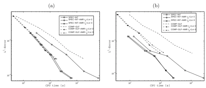
In this chapter, we apply the AMR technique to two different WENO schemes introduced in [23], namely to a WENO scheme implemented in a component-wise manner combined with global Lax-Friedrich flux vector decomposition (denoted by "COMP-GLF"), and alternatively for a WENO scheme applied in a characteristic (spectral) manner and which makes significant use of the interlacing property of the velocities v1,. However, SPEC-INT is significantly more accurate than COMP-GLF and is found to be even more effective than COMP-GLF in reducing numerical errors per CPU time [23].
Preliminaries
Sedimentation of polydisperse suspensions
Secular equation and hyperbolicity analysis
1.7) When m ≤ 2, the quantities (1.7) can be easily calculated and the analysis of hyperbolicity via the secular equation is much less involved than the discussion of the zeros of det(Jf(Φ)−λI) as was done in [12, 94] . For the special case of the MLB model with spheres of equal density, vi depends on the parameters p1 :=φ and p2 :=δTΦ.
Numerical schemes
SPEC-INT and COMP-GLF schemes
The key point is designed by the numerical flux ˆfi+1/2 so that the resulting scheme is (at least formally second-order) accurate and stable. For polydisperse sedimentation, exact Riemann solvers are out of reach, as the eigenstructure of the flux Jacobian is difficult to calculate.
Adaptive Mesh Refinement (AMR)
The networks corresponding to the different levels Gl, 1≤l≤L must be modified according to the actual flow characteristics. New cells are only included due to the addition of a few extra cells around each marked cell.
Numerical results
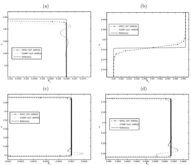
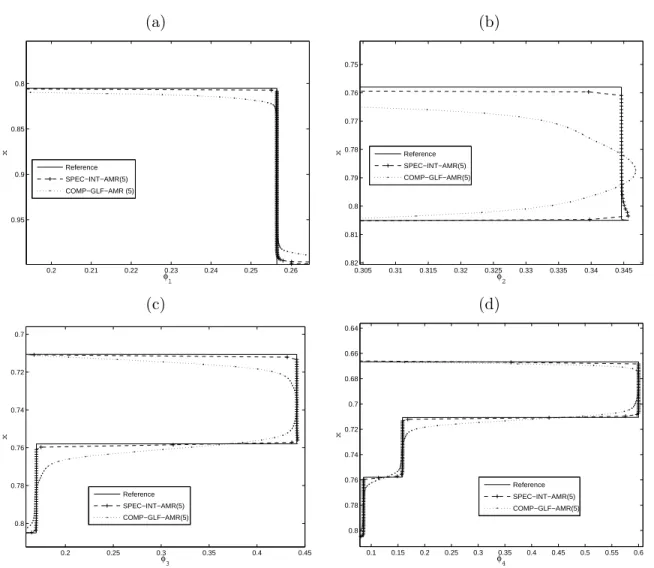
We observe that the CPU time and the percentage of memory allocated by the SPEC-INT-AMR and COMP-GLF-AMR codes decrease as N0 increases, as expected. However, we observe in Figures 1.2 that the COMP-GLF-AMR code produces spurious oscillations in the semi-constant part of the solution.
Also shown is the solution generated by SPEC-INT on a fixed grid with 1600 subintervals and the reference solution computed by SPEC-INT on a fixed grid with Nref = 12800. The reference solution was computed using the SPEC-INT scheme on a fixed grid with 12800 subintervals at timest= 400 s and t= 2500 s.

Conclusions of Chapter 1
Scope
The aim of this chapter is to design non-linear solvers for suitable regularizations of the systems that occur when implicit-explicit (IMEX) schemes are used for the efficient solution of initial-boundary value problems for (2.1) under the specific assumptions of diffusively corrected cinematic. The most important novelty of this chapter is the particular method of solving the non-linear systems that occurs with the implicit treatment of the degenerate diffusion term.
Related work
On the other hand, a multi-class version of the diffusion-corrected LWR model proposed by Nelson [81], which can also be understood as a diffusion-corrected version of the MCLWR traffic model [8, 113], is newly derived here. The IMEX Runge-Kutta scheme consists of a combination of the Runge-Kutta scheme with an implicit discretization of the diffusion term with an explicit discretization for the convective term.
Diffusively corrected multi-species kinematic flow models
Polydisperse sedimentation
In fact, following the pioneering work of Crouzeix [42], numerical integrators that deal implicitly with D(Φ) and explicitly with C(Φ) can be used with a time step constraint dictated by the convective term alone. Finally, we mention that many authors have proposed IMEX Runge-Kutta schemes for the solution of semi-discretized partial differential equations.
Hyperbolicity and parabolicity analysis for the polydisperse sedimentation
A new diffusively corrected MCLWR model (DCMCLWR model)
Now we wish to state sufficient conditions for the nonnegative parameters vmaxi ,τiandLinwhereB(Φ) has eigenvalues with positive real parts for all Φ∈ Dφmax. Thus, we cannot expect B(Φ) to have non-negative eigenvalues alone without further constraints and structural conditions between the parameters vimax,Li and τi. We recall that the system (2.1) is called the parabolic of a state Φ0 if the eigenvalues of B(Φ0) have non-negative real parts.
Numerical schemes
- Spatial discretization
- Boundary conditions
- Explicit schemes
- Implicit-explicit schemes
- IMEX Runge-Kutta schemes
Variants of the original MCLWR model (in the sense of [8, 113]) have been proposed and partially analyzed for highways with different road surface conditions, traffic flow in networks [63, 84] and basic stochastic diagrams (equivalent to speed functions ) [85]. Ngoduy and Tampere [87] study the influence of different reaction times (of a single driver class) in terms of the same model. Variants of the original MCLWR model (in the sense of [8, 113]) have been proposed and partially analyzed, for highways with different road surface conditions, traffic flow in networks [63, 84], basic stochastic diagrams (equivalent to functions of velocity vi) [85], and diffusive corrections modeling prediction lengths and reaction times [30, 32].
Implicit-explicit Runge-Kutta scheme
Nonlinear solvers
We perform a linearized stability analysis for the system (3.6) under the assumptions of the DCMCLWR model. For the L-RS scheme in Table 4.2, we see that the relative mass error over simulated time is small with a coarse grid and decreases with mesh refinement. As in other examples, we see in Table 4.2 that the percentage relative mass loss at simulation times decreases with mesh refinement.
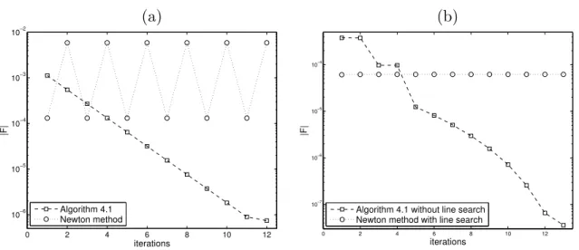
Newton-Raphson method with line search strategy
Numerical results
- Example 2.1: settling of a tridisperse suspension
- Examples 2.2 and 2.3: diffusively corrected kinematic traffic model
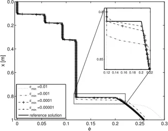
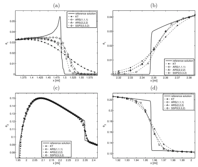
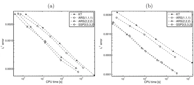
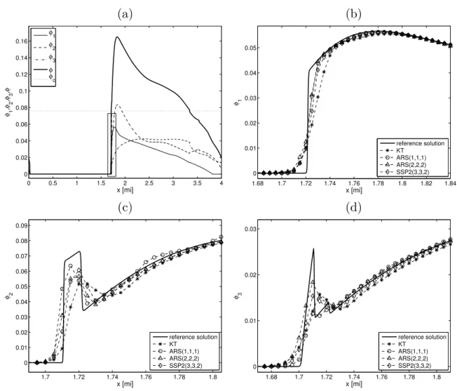
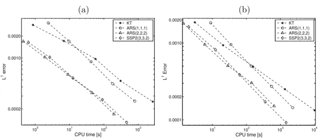
Careful observation of CPU times of the same scheme and resolution at different simulated times yields that the CPU time is not proportional to the simulated time. In Figure 2.8 we compare the results obtained with the KT, IMEX-RK schemes at simulated time T = 0.2 hours against the reference solution. Note that for the scheme IMEX-SSP2(3,3,2) and each fixed value of ε, the NR method requires a maximum of 3 iterations, but only one iteration is needed on average.

Derivation of the model of polydisperse sedimentation with compression
As in [12], we obtain an explicit formula for the slip velocities ui by solving the equations in (2.43) and choosing φi/α(Φ) = −d2iV(Φ)/(18µf) which is consistent with the Masliyah-Lockett- Fagot model. N, (2.44) where µf is the viscosity of the pure liquid, ie the respective species diameters, and the hindered settling factor V(φ) can be chosen as V(φ) = (1−φ)n−2 roach >2. The final model equations are the continuity equations of the solids and of the mixture.
Conclusions of Chapter 2
- Scope
- Related work
The MCLWR model is thus given by a strongly coupled system of nonlinear first-order conservation laws of the type We formulate, and partly evaluate, a stability criterion for the model (3.6) based on an analysis of the eigenvalues of the matrices. However, we demonstrate in Example 3.14 of Section 3.4.6 that the non-linearity of the diffusion terms in (3.6) together with the (mild) assumption V0(0) =V0(1) = 0 prevents this phenomenon from occurring.
Diffusively Corrected MCLWR model DCMCLWR
- The model equations
- Stability analysis
- DCLWR model with drivers having the same maximum speed
This would completely ruin the solution of the nonlinear system, because these oscillations would appear in all frequencies above ξ0. This discussion illustrates that satisfying the stability criterion determined by (3.14), namely that the pairwise distinct eigenvalues λ1,. This matrix is a perturbation of rank one of a multiple of the identity matrix I, and its eigenvalues are given by .
Parabolicity analysis
Numerical results
- Example 3.1 (DG model, N = 4, stable behaviour)
- Examples 3.2–3.5 (DG model, N = 2, unstable behaviour)
- Examples 3.6–3.8 (DG model, N = 2, mildly unstable behaviour)
- Examples 3.9–3.11 (GS model, N = 4 and N = 2)
- Examples 3.12 and 3.13 (DG model, N = 5, drivers having the same maxi-
- Example 3.14 (Daganzo’s test, N = 4)
In Figure 3.3 (a), we describe the stability region in the plane (φ1, φ2) (phase space), which corresponds to the points in which the real parts of the eigenvalues B(Φ) are positive. In particular, the oscillations seen in the numerical solution (see Fig. 3.6 (a, b)) are not artefacts caused by the numerical scheme. Figure 3.9 shows the stability region for the diffusion matrix B(Φ) and the instability region for the matrix M.
Conclusions of Chapter 3
- Scope
- Related work
Alternatively, one can construct numerical schemes that are easy to implement by exploiting the concentration-times-velocity form (4.2) of the fluxes, and exploiting that by (4.3) and (4.4) the functions are non-negative, bounded, and strictly decreasing. To explain the main idea, let us consider the continuity equation for the caseN = 1 of a single driver class. corresponding to the original LWR model [75, 92], where. and for ease of argument we assume in the scalar case that time is scaled such that vmax equals unity. Our proposal for the class of LR schemes for the MCLWR model is supported by a partial analysis of the L-AR schemes for N = 1, with the conclusion that under appropriate CFL conditions the L-AR schemes have total variation decreasing ( TVD) property and therefore converges to a weak solution and by a series of numerical experiments showing that the proposed schemes are competitive with newer schemes introduced in [24], see section 4.2.3.
Preliminaries
- Weak solutions and entropy admissibility
- Interlacing property of the MCLWR model
- Some simple difference schemes for the MCLWR model
In this chapter, we will not attempt to prove that any of the newly introduced schemes converge to an entropy solution, i.e., a weak solution satisfying (4.13). However, further support of the new schemes is provided by a heuristic argument based on the evaluation of a discrete analog of E(ρ) for the given numerical solutions, and for some examples involving (4.16), we will verify whether the numerical solution approximates the discontinuities that are consistent with (4.17). For ease of presentation, we will refer to Schemes 4 and 10 of [24] simply as “Scheme 4” in the remainder of the chapter.
Discretization of the Lagrangian step
Anti-diffusive schemes for the remap step
- Anti-diffusive schemes
- Choice of the numerical fluxes
- Lagrangian-anti-diffusive remap (L-AR) schemes, scalar case (N = 1)
- The multi-species case (N ≥ 1) and CFL condition
In the following [14] we denote this scheme for (4.9) by UBee and refer to the corresponding full L-AR scheme based on scheme (4.42) asL-UBee. Then we can obtain a numerical solution {ρn+1,−j }j∈Z after an evolution in a time interval of length ∆t, using scheme (4.26). Using this solution we solve equation (4.9) with scheme (4.31), where the value ¯Vjnstill must be determined in such a way that the resulting scheme is conservative.

Statistically conservative schemes
- Integral remap
- Random sampling remap, scalar case (N = 1)
- Random sampling remap, multiclass case (N > 1)
- Lagrangian-random sampling (L-RS) scheme
To define ρn+1j without introducing numerical diffusion, we follow a Glimm-type random sampling strategy [55]. Reassign random sampling step. For N = 1, we use the two-state-per-cell random sampling step (4.53) to advance the solution to n+1. We then perform the tristate-per-cell random sampling step (4.60) to obtain a numerical solution{ρn+1j }j∈Z fort=tn+1.
Numerical results
- CFL condition, errors, and entropy test
- Example 4.1: N = 1, linear velocity
- Example 4.2: N = 1 exponential velocity
- Example 4.3: N = 5, linear velocity
- Examples 4.4 and 4.5: N = 9, exponential velocity
Enlarged images of relevant parts of the numerical solutions in figure 4.11 for some selected species are shown in figures 4.12 and 4.13. However, the L-RS scheme is more diffuse than Scheme 10, and in Figure 4.13 we observe a delay in the approximation of the shock wave. In figure 4.15 we show the total entropy as a function, often we observe that the function (4.61) is not increasing in time.

Conclusions of Chapter 4
Por ello, para motivar el uso de esquemas numéricos que requieran menor esfuerzo computacional y/o esquemas que sean sencillos de implementar y que no requieran el uso de la información característica del modelo, en la tesis se motivan diferentes alternativas de esquemas numéricos la resolución de este tipo de modelos. Las simulaciones para N = 4 y N = 7 mostraron que los esquemas numéricos con AMR requieren menos esfuerzo computacional que los esquemas sin refinamiento adaptativo. Los resultados numéricos indicaron que estos esquemas son competitivos con respecto a otra variedad de esquemas, excepto que no requieren el uso de la información de características de flujo.
Trabajo Futuro
Implicit-Explicit Runge-Kutta Schemes for Hyperbolic Systems and Kinetic Equations in the Diffusion Limit.SIAM J. Anti-diffusive and random-sampling Lagrangian remap schemes for the Lighthill-Whitham-Richards multiclass traffic model.Preprint 2013-14 , Centro de Research en Ingenier'ıa Matem'atica, Universidad de Concepci'on; (submitted). Stochastic traffic flow modeling and simulation: asymmetric single exclusion process with Arrhenius look-ahead dynamics.SIAM J.