MULTIVARIATE GRAM-CHARLIER DENSITIES

MULTIVARIATE GRAM-CHARLIER DENSITIES

ESTHER B. DEL BRIO TRINO-MANUEL ÑÍGUEZ

JAVIER PEROTE

FUNDACIÓN DE LAS CAJAS DE AHORROS DOCUMENTO DE TRABAJO

Nº 381/2008

De conformidad con la base quinta de la convocatoria del Programa de Estímulo a la Investigación, este trabajo ha sido sometido a eva- luación externa anónima de especialistas cualificados a fin de con- trastar su nivel técnico.

La serie DOCUMENTOS DE TRABAJO incluye avances y resultados de investigaciones dentro de los pro- gramas de la Fundación de las Cajas de Ahorros.

Las opiniones son responsabilidad de los autores.

MULTIVARIATE GRAM-CHARLIER DENSITIES^*

Esther B. Del Brio

^**

Trino-Manuel Ñíguez

⁺

Javier Perote

⁺⁺

University of Salamanca Westminster University Rey Juan Carlos University

Abstract

This paper introduces a new family of multivariate distributions based on Gram-Charlier and Edgeworth expansions. This family encompasses many of the univariate seminonparametric densities proposed in the financial econometrics as marginal distributions of the different formulations. Within this family, we focus on the specifications that guarantee positivity so obtaining a well-defined multivariate density. We compare different "positive" multivariate distributions of the family with the multivariate Edgeworth-Sargan, Normal and Student’s t in an in- and out-sample framework for financial returns data. Our results show that the proposed specifications provide a quite reasonably good performance being so of interest for applications involving the modelling and forecasting of heavy-tailed distributions.

Keywords: Multivariate distributions; Gram-Charlier and Edgeworth-Sargan densities;

MGARCH models; financial data.

JEL classification code: C16, G1.

* Financial support from the Spanish Government through project SEJ2006-06104/ECON is gratefully acknowledged.

** Dept. de Administración y Economía de la Empresa. Campus Miguel de Unamuno. 37007 Salamanca (Spain).

Tel: +34-923294400, Ext. 3515. Fax: +34-923294715. E-mail: [email protected].

+ Dept. of Economics, Westminster Business School, University of Westminster, 35 Marylebone Road, NW1 5LS London, UK. Tel: +44 (0) 22 7911 5000, fax: +44 (0) 22 79115839. Email: [email protected].

++ Corresponding Author: Dept. de Fundamentos del Análisis Económico. Campus de Vicálvaro. 28032 Madrid (Spain). Tel: +34-914887684. Fax: +34-914887780. E-mail: [email protected].

1. Introduction

The Gram-Charlier and Edgeworth expansions were established at the end of the 19th century and the beginning of the 20th century by Edgeworth (1896, 1907) and Charlier (1905). Since then, these expansions have been used in many fields from mathematics or statistics to physics, but it was Sargan in the 70s who brought these expansions into econometrics - Sargan (1975, 1976). More recently, the literature on this topic has increased from both theoretical studies - e.g. Nishiyama and Robinson (2000), Velasco and Robinson (2001) and Nabeya (2001) - and applications in finance to fit the heavy-tailed distribution of high-frequency asset returns - Corrado and Su (1996), Mauleón and Perote (2000) and Verhoeven and McAleer (2004), among others.

The latter articles provide evidence of the good performance of these distributions, besides of, the widely known nonpositivity curse that they present when they need to be truncated in practical applications, as firstly highlighted by Barton and Dennis (1952) and Draper and Tierny (1972). Different solutions has been proposed to this problem in univariate contexts by authors such as Gallant and Nychka (1987), Gallant and Tauchen (1989), Jondeau and Rockinger (2001), Ñíguez and Perote (2004) and Leon et al. (2005).

On the other hand, the multivariate context may be of greater interest to explore the possible gains in in-sample fit and forecasting when accounting for the joint distribution of correlated variables. For such purposes different approaches have been proposed, including:

Multivariate Skewed Normal (Azzalini and Dalla Valle, 1996), Multivariate Student's t (Kotz and Nadarajah, 2004), Multivariate Weibull (Malevergne and Sornette, 2004), Kotz-type distributions (Olcay, 2005) and copula methods (e.g., Xiaohong et al., 2006) and multivariate GARCH models (Bauwens et al., 2005). Nevertheless, to the knowledge of the authors, the Gram-Charlier and Edgeworth expansions have scarcely been studied in a multivariate context.

¹

Recently, Perote (2004) has proposed a closed form for a multivariate density based on the so-called Edgeworth-Sargan distribution (ES henceforth). The resulting density, called Multivariate ES (MES henceforth), showed a good performance to fit the multivariate distribution of financial returns.

²

But, as the ES, the MES distribution also presents the problem of not being positive for all values of the parameters in the parametric space.

³

The main aim of this article is to shed some light on this issue by providing a family of positive multivariate Gram-Charlier distributions that generalise the univariate positive Gram-Charlier distributions proposed in the literature.

The remainder of the article is structured as follows. Section 2 deals with the definitions of the multivariate Gram-Charlier family of densities. Section 3 tests the performance of the proposed densities through an empirical application for financial data, and Section 4 presents the main conclusions and suggests possible lines for further research.

2. Multivariate Gram-Charlier Densities

In this section we propose a general multivariate family of distributions based on the seminonparametric (SNP henceforth) density approach derived from the Edgeworth or Gram- Charlier expansions. This family encompasses most of the univariate ES used in the literature

1 See, e.g., Henery (1981) for a particular case of uncorrelated variables applied to model disease transmission.

2 See also Perote and Del Brio (2003) for applications of the MES distribution to estimate Value-at-Risk (VaR henceforth) measures.

3 Note that we refer to the ES distribution as an already truncated Edgeworth expansion.

to model and forecast high-frequency financial returns for risk management purposes. The

"standardised" Multivariate Gram-Charlier (MGC hereafter) family of densities is defined in terms of the "standardised" multivariate Normal (MN hereafter) density, G(

•

), - i.e. with zero mean and unitary variance for all its marginal densities, g(

•

), and correlation coefficients denoted by ρ

ij

∀i,j=1,2,…,n; i ≠ j - and the so-called Hermite polynomials, H

s

(

•

), as given in the definition below.

⁴

Definition 1 A random vector X=[x1

,x

2

,…,x

n

]′

∈ℜⁿ

belongs to the MGC family of distributions if it is distributed according to the following density function,

( )

⎭⎬⎫

⎩⎨

⎧

⎭⎬

⎫

⎩⎨

⎧ + +

= +

∏ ∑

=

=

n i

i i i i n

i

i x A x

x c n g

X n G

X F

1 1

) ( h )' ( 1 h )

1 ( ) 1 1 (

1

, (1)

where A

i

is a matrix of order (q+1),

⁵

h(x

i

)′=[1,H

1

(x

i

),…,H

q

(x

i

)]′ ∈ℜ

^q+1

, H

s

(x

i

) stands for the s- th order Hermite polynomial, described in equation (2),

⎪⎪

⎩

⎪⎪⎨

⎧

− −

− −

=

∑

∑

−

=

−

=

−

2 / ) 1 (

0

2 2

/

0

2

odd is if )!

2 (

! 2 ) !

1 (

even is if )!

2 (

! 2 ) !

1 ( )

( _s

i i

i s i i s

i i

i s i i i

s

i s s i x s

i s s i x s x

H

(2)

and c

i

is the constant such that

∫

= _{i i i i i}

i

x A x g x dx

c h ( )' h ( ) ( ) . (3)

Note that the MGC family of functions straightforwardly integrates up to one and represents density functions provided that A

i

is a positive definite matrix, ∀i=1,2,…,n. An interesting and simple case arises when this matrix admits the following decomposition, A

i

=d

i

d

i′, where di

=[1,d

i1

,…,d

iq

]′ ∈ℜ

^q+1

∀i=1,2,...,n contains the density parameters of the i-th density dimension. For this particular case, a positive version of the MGC density, hereafter named as MGCI, can be defined as in equation below, (4).

( )

⎪⎭

⎪⎬

⎫

⎪⎩

⎪⎨

⎧

⎥⎦

⎢ ⎤

⎣

⎡ +

⎭⎬

⎫

⎩⎨

⎧ + +

= +

∏ ∑ ∑

= =

=

n i

q s

i s is i

n i

i

I d H x

x c n g

X n G

X F

1

2

1 1

) ( 1 1

) 1 (

) 1 1 (

1

, (4)

For this density, and based on the well-known orthogonality properties given in equations (5), (6) and (7),

⁶

∫ ^H

^s

^{( x}

ⁱ

^{) H}

^j

^{( x}

ⁱ

^{) g ( x}

ⁱ

^{) dx}

^{i =}

^{0 if s}

^≠

^{j (5)}

∫ ^H

^s

^{( x}

ⁱ

^{) H}

^j

^{( x}

ⁱ

^{) g ( x}

ⁱ

^{) dx}

^{i =}

^{s ! if s}

⁼

^{j (6)}

4 Note that although we define the "standardised" MGC densities in terms of Gaussian densities with unitary variance, the resulting distributions do not have unitary variance, since variances, as the rest of the density moments, depend on the whole set of density parameters.

5 Note that without loss of generality we have considered that for all dimensions the Gram-Charlier (type A) expansions are truncated at the same order q.

6 See Kendall and Stuart (1977) for further details about the Hermite polynomials properties.

∫ ^H

^s

^{( x}

ⁱ

^{) g ( x}

ⁱ

^{) dx}

^{i =}

^{0 for every s (7)}

it can be straightforwardly proved that:

(i) The constant that weights the squared sum of Hermite polynomials for every variable x

i

(see Proof 1 in the Appendix) is

∫ ∑ ∑

=

=

+

⎥ =

⎦

⎢ ⎤

⎣

⎡ +

= ^q

s is

i i q

s is s i

i

d H x g x dx d s

c

1 2 2

1

! 1

) ( ) (

1 (8)

(ii) The density integrates up to one (see Proof 2 in the Appendix).

(iii) The marginal density for variable x

i

is a mixture of a univariate normal and a univariate SNP density of the type recently analysed in Leon et al. (2005, 2006), as shown in equation (9) (see Proof 3 in the Appendix).

) ( ) ( ) 1

1 ( ) 1 1 ( )

(

2

1 i

q

s is s i

i i

i

I

d H x g x

c x n

n g x n

f

⎥

⎦

⎢ ⎤

⎣

⎡ + + +

= +

∑

=

(9) Note that the MGCI distribution overcomes the aforementioned nonpositivity problem that may arise in applying the MES density in Perote (2004), equation (10).

⁷

Therefore, the MES is not nested in the “positive” MGC family of distributions but it can be consider as a precursory of the family since it is also based on Gram-Charlier Type A expansions.

( )

⎭⎬⎫

⎩⎨

⎧

⎭⎬

⎫

⎩⎨ +⎧

=

∏ ∑∑

= =

=

n i

q s

i s is n

i i

ES X G X g x d H x

F

1 1

1

) ( )

( )

(

(10)

On the other hand, the MGCI density may also be interpreted as a multivariate generalisation of Gallant and Nychka's methodology.

⁸

An interesting feature of the MGC family of densities proposed in this paper is its general formulation since it may encompass many different "positive" multivariate densities.

For instance, another possible alternative is the density defined in equation (11) below, which is a special case for A

i

= diag{1,d

i1

, …, d

iq

} and we denote as MGCII,

( )

⎭⎬⎫

⎩⎨

⎧ ⎥

⎦

⎢ ⎤

⎣

⎡ +

⎭⎬

⎫

⎩⎨

⎧ + +

= +

∏ ∑ ∑

= =

=

n i

q s

i s is i

n i

i

II

d H x

x c n g

X n G

X F

1 1

2 2

1

) ( 1 1

) 1 (

) 1 1 (

1 . (11)

For this density the scaling constants, c

i

∀i=1,2,...,n, are also those in equation (8) but its marginals, equation (11), are mixtures of a univariate normal and the univariate positive ES (PES) of Ñíguez and Perote (2004).

7 Note that for the maximum likelihood estimates the MES is necessarily positive and thus this density can be estimated in many applications by choosing accurate initial values, based on the estimates for its marginal densities that are distributed as the univariate ES in Mauleon and Perote (2000).

8 See Fenton and Gallant (1996) for a detailed analysis of the properties of the SNP densities defined when truncating Edgeworth and Gram-Charlier expansions.

) ( ) ( ) 1

1 ( ) 1 1 ( )

(

1

2 2

i q

s

i s is i

i i

II d H x g x

c x n

n g x n

f ⎥

⎦

⎢ ⎤

⎣

⎡ + + +

= +

∑

=

(12) Furthermore, the MGCII cumulative distribution functions (cdf hereafter) can be easily worked out as shown in equation (13) - see Proof 4 in the Appendix, and consequently, they can be straightforwardly implemented for risk management purposes, either for modelling and forecasting credit risk, portfolios VaR or shortfall probabilities. The multivariate cdf of the MGCI can be obtained analogously in terms of the cdf of univariate N(0,1) and univariate SNP – see Leon et al. (2006) – distributions.

[ ] ∫

−∞

∫

−∞ +

= +

≤

≤ _{n n} ^{a an}

G X dx dx

_n

a n x a x

ob

1 1 L L

( )

1L

1 , 1

,

Pr

¹

∑ ∫ ∑ ∑ ∏∫

=

−

≠= −∞

∞

− =

−

= − − − ⎥

⎦

⎢ ⎤

⎣

⎡

− − + ⁿ

i

n

s jj

a

j j

a q

s s

k s k i s k i

is i

i i

i

j

i

H a H a g x dx

k s d s c

a dx g

x g

1

1

1 1 1

0 1

2

( ) ( ) ( )

)!

( ) !

) (

( (13)

The MGC densities also admit the specification of GARCH-type processes (Engle (1982) and Bollerslev (1986)) to explain the dynamics of their conditional moments.

Particularly, the conditional variances, k

_it²

, are introduced by considering transformations of the type r

t

= Λ

t

X where Λ

t

= diag{ k

1t

, k

2t

,..., k

nt

}.

⁹

In the next section we test the performance of the bivariate versions of these new densities in comparison with the MES, the MN and the Multivariate Student’s t (MST hereafter) through an empirical exercise for stock returns.

Specifically we consider the following specification

¹⁰

t

t

u

r

=

μ (

Φ

)

+

(14)

)) ( , 0

1 ( _t α

t

t MGC

u Ω₋ ≈ Λ

. (15)

3. Empirical examples

3.1. Data estimation and in-sample analysis

The data used are daily returns of S&P500 and the Hang-Seng indices of the New York and Hong Kong Stock Exchange, respectively, r

_t

'

=

[ r

_1t

r

_2t

] , over the period December 19, 1991 to December 19, 2006 for a total of T=3,913 observations, obtained from Datastream. A plot and descriptive statistics of r

t

is presented in Figure 1.

Let the conditional distribution of r

t

, be either MN, MGCI, MGCII or MST

¹¹

with conditional mean and covariance matrix modelled according to equations (14) and (15), respectively. In particular we use AR(1) and GARCH(1,1) time-varying structures for modelling the conditional means and variances as shown in equations (16) and (17).

9 Note that this model is a case of the constant conditional correlation (CCC henceforth) model of Bollerslev (1990), where the constant correlations coefficients are those ρij included in the "standardised" MN of the MGC densities.

10 It must be noted that the variance and covariance matrix of rt is Λt(α)Σt (d, ρ)Λt(α) where Σt(d,ρ) is the variance and covariance matrix of the MGC process.

11 Specifically we use Prucha and Kelejian’s (1984) version of the MST – see also Kotz and Nadarajah (2004) for other MST alternatives.

1,2.

1

, 1

0 + ∀ =

= _{i i}

r

_it−

i

it

φ φ

μ (16)

1,2.

2

1 , 2 2

1 , 1 0

2 = + u ₋ + k ₋ ∀i=

k_it α_i α_{i it} α_{i it}

(17)

Figure 1: S&P 500 and Hang-Seng indices daily returns. Sample: 19/12/1991 - 06/06/2005

(observations 3,513). Out-of-sample: 07/06/2005 - 19/12/2006 (observations 400).

The estimation procedure is carried out in two steps using an in-sample window of S=3,513 observations. Firstly, the AR(1) process is estimated by ordinary least squares and, secondly, covariance matrix coefficients and density function parameters are estimated by (quasi)-maximum likelihood ((Q)ML) using the AR(1) residuals from the first step. Robust QML covariance estimators are calculated by means of Bollerslev and Wooldridge (1992) formula. The Hermite polynomials expansions were truncated in the 8

^th

term according to accuracy criteria. Moreover, the odd parameters of the expansions were constrained to zero because they were found not to be statistically significant.

¹²

Tables 1 and 2 display the estimates for the parameters of the bivariate densities when variances are assumed to be either constant or follow a GARCH(1,1), respectively.

¹³

Under

12 There is evidence in favour of the existence of skewness in financial returns when conditional skewness is considered, e.g. Harvey and Siddique (1999). Nevertheless, for all the analysed cases the MGC densities where found to be unconditionally symmetric. Moreover, the introduction of conditional patterns for moments other than the variance (e.g. for skewness or kurtosis) when positivity constraints are imposed in Gram-Charlier expansions is still an open question.

13 It is worth mentioning that the estimation of the joint distribution of a larger number of assets is not an extremely difficult task since the number of parameters only increases proportionally to the number of

the former assumption the scale parameter of variable i is denoted by k

i

and under the latter α

ij

∀j=0,1,2 and ∀i=1,2 stand for the parameters of the GARCH(1,1) model used for the

conditional variances. Moreover, φ

ij

∀j=0,1 are the intercept and the slope, respectively, of the AR(1) process used to capture the conditional mean of every variable i.

¹⁴

The rest of the parameters displayed in both tables follow the same notation used throughout the paper.

dimensions. Therefore, the more complex structures can be estimated by implementing algorithms that use the estimates for the marginal densities as initial values for the multivariate distribution.

14 Note that the AR(1) coefficients are not displayed in Table 2 since they are the same as those in Table 1.

Both tables include the corresponding t-statistic for each parameter (in parentheses), the log-likelihood value (lnL) and the Schwarz Bayesian Information Criterion (BIC), defined as BIC=−lnL+pln(S)/2 where p stands for the number of the parameters of the model. As a first orientative approach,

¹⁵

according to these accuracy criteria the MES seem to outperform the other distributions and the performance of the distributions that incorporate time-varying variances are also superior to their unconditional counterparts. Regarding to the parameter estimates most of them are significant at the 5 per cent confidence level, confirming the fact

15 Note that the comparison in terms of these criteria is only valid for nested distributions.

that the proposed models seem to be accurate fits of the density underlying the S&P500 and Hang-Seng indices. Nevertheless the interpretation of the parameters of the MGC densities requires a complete study of the moments of every distribution. For example, ρ

ij

does not capture exactly the correlation among both indices, which explains the significant differences of this parameter among the estimated densities.

¹⁶

The stationarity conditions of the GARCH processes in all the distributions except the MN are also slightly different from the usual ones as well.

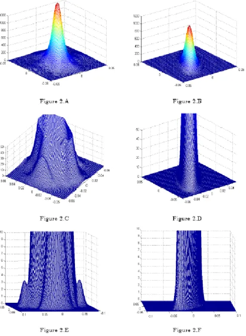
¹⁷

Figure 2: Fitted MGCII density of the S&P500 and the Hang-Seng indices returns for

different ranges and domains.

16 Specifically for the analysed MGC densities the Pearson’s correlation coefficient can be obtained as )

1 ( / _{1 2}

12

σ σ

n+

ρ

where

σ

₁ and

σ

₁ are the standard errors of every variable obtained from the corresponding univariate Gram-Charlier marginal densities.

17 See See Ñíguez and Perote (2004) for an example of the GARCH(1,1) stationarity conditions for the particular case of the univariate PES density.

Finally, and for the purpose of illustrating the performance of this family of distributions, the fitted MGCII density with constant variances (Table 1) is depicted in Figure 2. This Figure includes the pictures for the fitted MGCII (left plots: Figures 2.A, 2.C and 2.E) compared to the corresponding fits under the MN (right plots: Figure 2.B, Figure 2.C and Figure 2.F) for different ranges and domains. Particularly, Figures 2.A and 2.B represent the whole domain of the functions, and the rest of the figures illustrate details of the distributions tails. It is noteworthy the fact that the MGCII is capable of capturing different jumps in the probabilistic mass (see Figure 2.C) whilst for the same range the MN density decreases smoothly (see Figure 2.D). Furthermore, the MGCII captures more accurately the leptokurtic density behaviour since it assigns positive probability to areas in the tails where the MN does not (see Figures 2.E and 2.F). This improvement in the accuracy of the MGCII is due to its flexibility to incorporate the whole shape of the density by means of a larger number of parameters than other distributions such as the MN.

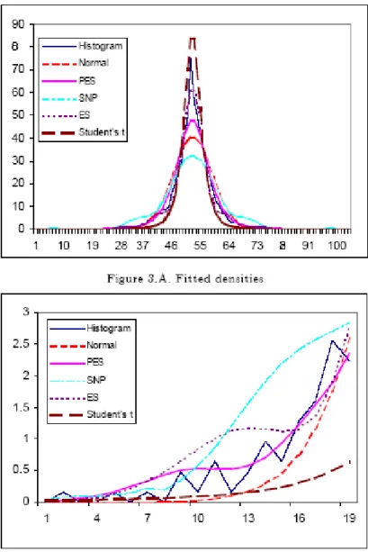
Figure 3: Fitted marginal density of S&P500 index computed from the estimated MN, MES

and MGCII compared to the histogram of the data.

These findings can be also illustrated by depicting the marginal densities of every variable computed from the estimates for the multivariate distributions. Figure 3 includes the fitted marginal density for S&P500 under different specifications (MN, MST, MES, MGCI and MGCII) in comparison to the histogram of the data. Figure 3.A represents the densities for the whole domain whilst Figure 3.B includes only the distributions left tails. From these pictures it is clear that although the MES seems to capture more accurately the sharply peaked density behaviour, the MGCII outperforms the other specifications in the tails. Specifically this distribution is clearly superior to less flexible distributions such as the MN and MST

¹⁸

and other seminonparametric alternatives (e.g. the MES or the MGCI). Therefore in the next section we study the out-of-sample performance of the MGCII as a representative well- behaved MGC distribution.

3.2. Density forecasting

In this section we test the performance of the MGC densities to forecast the full density of the portfolio and compare the forecasts with those of a MN model by using the methodology in Diebold et al. (1998, 1999) and Davidson and MacKinnon (1998). The application of this methodology in a multivariate framework is based on cumulative marginal and conditional distribution functions (cdf), evaluated at the forecasted standardised AR(1) residuals, u ˆ

_i,_t+1 =

( r

_i,_t+1−

μ ˆ

_i,_t+1

) k ˆ

_i,_t+1 ∀i=1,2, through the out-of-sample period (N=400

observations). The resulting so-called probability integral transforms (PIT hereafter) sequences, labelled p

1t

, p

2t,

p

_1⏐2,t

and p

_2⏐1,t

are i.i.d. U(0,1) under correct density specification,

∫

−∞⁺ + + + ∀ =

= ^{uˆi,t 1} _{i,t 1}( _{i,t 1}) _{i,t 1} 1,2

it f u du i

p

(18)

2 , 1 , )

(

) , ) (

( , 1

1

, , 1

1 ,

ˆ

1 , 1 , 1 ,

ˆ ˆ

1 , 1 , 1 , 1 , ˆ 1

1 , 1 1 , ,

, = = ∀ =

∫

∫ ∫ ∫

⁺

+ +

+

∞

− + + +

∞

− −∞ + + + + +

∞

− + + + i j

du u f

du du u

u du f

u f

p it

t

i jt

t i

u

t i t i t j

u u

t j t i t j t i u t

t i t t i j i t

j

i

(19)

where f

it

(

•

),f

_i⏐j,t

(

•

) and f

t

(

•

) denote marginal, conditional and joint distributions, respectively.

Moreover since p

it

is also interpreted as the p-value corresponding to the quantile u ˆ

_i,t+1

of the forecasted density we use the p-value plot methods in Davidson and MacKinnon (1998) to compare the models forecasting performance.

¹⁹

So, if the model is correctly specified the difference between the cdf of p

it

and the 45º line should tend to zero asymptotically. The empirical distribution function of p

it

can be easily computed as,

∑

=

≤

= ^N

t

l it l

p

p y

y N P

it

1

) (

1 1 )

ˆ ( , (20)

18 Note that, as pointed by Mauleon and Perote (2000), the degrees of freedom of the MST might be understated in an attempt to capture both the sharp peak and heavy tails with only this parameter. This fact explains the misspecified tail behaviour of the MST.

19 Davidson and MacKinnon (1998) used this method to compare the size and power of hypothesis tests, while following Fiorentini et al. (2003) we use it to discriminate among alternative models according to their performance for forecasting the full density.

where 1(p

it ≤

y

l

) is an indicator function that takes the value 1 if its argument is true and 0 otherwise, and y

l

is an arbitrary grid of l points.

²⁰

Alternatively, the p-value discrepancy plot (i.e. plotting

Pˆ_pit(y_l)−y_l

against y

l

) can be more revealing when it is necessary to discriminate among specifications that perform similarly in terms of the p-value plot (see Fiorentini et al., 2003). Consequently, under correct density specification, the variable

l l

p y y

Pˆ _it( )−

must converge to zero.

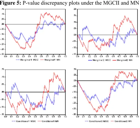
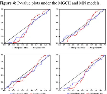
Figure 4: P-value plots under the MGCII and MN models.

Figure 5: P-value discrepancy plots under the MGCII and MN models.

20 We use the following l=215 points grid, yl = 0.001,0.002,...,0.01,0.015,...,0.99,0.991,...,0.999 since it highlights the goodness-of-fit in the distribution tails.

In Figures 4 and 5 we plot the marginal and conditional cdf for the PIT series of u ˆ

_i,t+1

,

∀i=1,2, under either MN (red line) or MGCII (blue line). We observe that the MGCII model

provides a reasonably good performance for forecasting the full density of the portfolio and clearly overcomes the MN model commonly used in financial applications.

4. Concluding remarks

This paper introduces a family of multivariate distributions based on Edgeworth and Gram-Charlier expansions. This family encompasses most of the univariate densities proposed in financial literature (e.g. the so-called Gram-Charlier, Edgeworth-Sargan or Positive Edgeworth-Sargan), which can be obtained as the marginal densities of the different densities nested in this family. Therefore, the MGC densities inherit the properties of their univariate precursories in terms of flexible parameter structure to accurately represent all the characteristic features of most high-frequency financial variables (i.e. thick tails, sharp peak, asymmetries, conditional heteroskedasticity, etc.). Within this family, the specifications that are positive for all the values of the parametric space (and are thus properly defined) merit particular interest. We provide some examples of positive multivariate densities overcoming the deficiencies of the MES density, which can be understood as applications of the Gallant and Nychka (1987) methodology to the multivariate framework. The performance of these densities is compared to fit and forecast the full density of a portfolio of asset returns, and it is found that they perform quite satisfactorily and are superior to the MN, the most commonly used distribution in financial risk management.

Within the multivariate densities based on Edgeworth and Gram-Charlier expansions the MES seems to be more accurate than other positive but more restrictive types of MGC distributions. This evidence highlights the fact that "positive Gram-Charlier expansions" can be adequate representations not only for univariate but also for multivariate densities, but at the cost of a loss of accuracy when compared to other cases (e.g. MES) that do not impose positivity a priory. Nevertheless, it must be noted that the MES has several disadvantages compared to MGCI or MGCII including: (i) it requires a more careful selection of initial values (or even the implementing of parameter constraints) to avoid the problems caused by possible negative values, (ii) the estimates do not guarantee positivity for other estimation techniques further than the maximum likelihood and (iii) in some contexts (such as when estimating the density recursively to compute a large number of forecasts) this distribution might give rise to problems of convergence, specifically if the data contain a large number of outliers. Moreover, we show that the MGCII data fits in the tails can be superior to those obtained by the MES. Therefore the choice among the different possibilities within the family depends on other empirical or econometric considerations rather than merely on accuracy issues.

This paper opens a hopefully fruitful line of research providing general formulations

for MGC densities, and showing evidence of their reasonably good in- and out-sample

performance through an empirical application. These results suggest that further research

seems worthwhile to investigate the model performance for other financial applications, as

e.g. asset pricing or credit and market risk forecasting.

Appendix

This appendix includes the proofs of some properties of the MGC densities.

Particularly, the constant that makes both the MGCI and the MGCII densities integrate up to one, the marginal densities of MGCI distribution and the cdf for the MGCII are derived. The corresponding proofs for other multivariate densities of the same family can be obtained analogously.

Proof 1:

∫ ∫ ∑ ∑ ∫

=

=

=

⎥ +

⎦

⎢ ⎤

⎣ + ⎡

= ^q

s

i i i s is i

i q

s

i s is i

i

i

g x dx d H x g x dx d H x g x dx

c

1 2

1

) ( ) ( 2

) ( ) ( )

(

∫ ∑ ∑ ∑ ∫

∫

= = =

= +

⎥ =

⎦

⎢ ⎤

⎣ + ⎡

= ^q

s

i i i j i s q

j

ij is i

i q

s

i s is i

i

dx d H x g x dx d d H x H x g x dx

x g

1 1

2

1

) ( ) ( ) ( 1

) ( ) ( )

(

∑ ∫

₌ ^{= +}

∑

₌

+

= ^q

s is

q

s dis Hs xi g xi dxi d s

1 2 1

2

2 ( ) ( ) 1 !

1

Proof 2:

∫ ∫

∫ ∫

^L

^F

^I

^{( X ) dx}

^1L

^dx

^{n =}

_n ¹

₊

₁

^L

^{G ( X ) dx}

^1L

^dx

^{n +}

∑∫ ∫ ∏ ∑

= = =

⎪⎭ =

⎪⎬

⎫

⎪⎩

⎪⎨

⎧

⎥⎦

⎢ ⎤

⎣

⎡ +

⎭⎬

⎫

⎩⎨

⎧ + + ⁿ

i

n q

s

i s is i

n i

i d H x dx dx

x c

n ₁ g ¹

2

1 1

) ( 1 1

) 1 (

1 L L

1 1 1

) 1 ( 1 1

) 1 (

1 1 1

1

2

1

+ = + +

⎥ =

⎦

⎢ ⎤

⎣

⎡ + + +

= +

∑ ∫ ∑

= =

n

n x n

H c d

x n g

n

n i

q s

i s is i

i

Proof 3:

∫ ∫

∫ ∫

⁼ ₊ ⁺

= _{I i− i+ n i− i+ n}

i

I

G X dx dx dx dx

dx n dx

dx dx X F x

f

L 1L 1 1L L

( )

1L 1 1L

1 ) 1

( )

(

∫∏

∑

⎥

∫

⁺

⎦

⎢ ⎤

⎣

⎡ + + +

≠= − +

=

n

i jj

n i

i j

q s

i s is i

i

dx dx

dx dx x g x

H d x

c g

n ₁ ^{1 1 1}

2

1

) ( )

( 1

) ) (

1 (

1 L L L

⎥ =

⎦

⎢ ⎤

⎣

⎡ +

⎪⎭

⎪⎬

⎫

⎪⎩

⎪⎨

⎧

+ +

∑ ∫ ∫ ∏ ∑

≠= − +

≠ =

= n

i jj

n i

i q

s

j s js n

i hh

j i

i

g x d H x dx dx dx dx

x c

n g

₁ ^{1 1 1}

2

1 1

) ( 1

) 1 (

) ) ( 1 (

1

L L L

+ = + −

⎥⎦

⎢ ⎤

⎣

⎡ + + +

+ +

∑

=

) 1 ( ) 1

( 1

) ) (

1 ( ) 1 1 (

1

²

1

i q

s

i s is i

i

i

g x

n x n

H d x

c g x n

n g

2

1

) ( 1

) ) (

1 ( ) 1

1 (

⎥

⎦

⎢ ⎤

⎣

⎡ + + +

= +

∑

= q s

i s is i

i

i

g x d H x

c x n

n g

n

Proof 4:

+ +

=

∫ ∫

∫ ∫

−∞ −∞ −∞ −∞

1 1

1

1

( )

1 ) 1

(

^{a a} _n

a a

n II

n

n

G X dx dx

dx n dx X

F

L L L

L

∫

−∞

∫ ∏

−∞

∑

=

∑

=

=

⎭ =

⎬⎫

⎩⎨

⎧ ⎥

⎦

⎢ ⎤

⎣

⎡ +

⎭⎬

⎫

⎩⎨

⎧

+ + ¹ ₁

1 1

2 2

1

) ( 1 1

) ) (

1 (

1

^a

n n

i

q s

i s is i

a n

j

i

d H x dx dx

x c n g

n L

L

∑ ∫ ∑ ∏∫

∫ ∫

₌

≠= −∞

∞ =

−

∞

− −∞ =

⎥⎥

⎥

⎦

⎤

⎢⎢

⎢

⎣

⎡

⎥⎦

⎢ ⎤

⎣

⎡ + + +

+ + ⁿ

i

N

i jj

a

j j i

q s

i s is i

a i a

n

a_{n i j}

dx x g dx

x H d x

c g dx n

dx X

n G

_{1 1 1}

2 2

1

1 ( ) 1 ( ) ( )

) 1 ( ) 1

) ( 1 (

1

¹

L L

+ +

=

∫ ∫

−∞ −∞

1

)

1

1 (

1

^{a a}

n

n

G X dx dx

n

L L

∑

₌

∫ ∑ ∑ ∏∫

≠= −∞

=

−

= − − −

∞

− ⎥⎥⎥

⎦

⎤

⎢⎢

⎢

⎣

⎡

⎥⎦

⎢ ⎤

⎣

⎡

− −

+ + ⁿ

i

n

i jj

a

j j q

s s k

i k s i k s is

a

i i i

i

j

i H a H a g x dx

k s d s c

a dx g

x

n 1 g 1 1

1

0

1

2 ( ) ( ) ( )

)!

( ) !

) ( ) (

1 (

1

- see Ñíguez and Perote (2004) for the details about the cdf for every marginal density of the PES distribution.

References

Azzalini, A. and A. Dalla Valle, 1996. The Multivariate Skew Normal Distribution.

Biometrika, 83, 715-726.

Barton D.E. and K.E.R. Dennis, 1952. The Conditions under which Gram-Charlier and Edgeworth Curves are Positive Definite and Unimodal. Biometrika, 39, 425-427.

Bauwens, L., S. Laurent and J. V. K. Rombouts, 2005. Multivariate GARCH Models: A Survey. Journal of Applied Econometrics, 21, 79-109.

Bollerslev, T., 1986. Generalized Autoregressive Conditional Heteroskedasticity. Journal of Econometrics, 31, 307-327.

Bollerslev, T., 1990. Modelling the Coherence in Short-Run Nominal Exchange Rates: a Multivariate Generalized ARCH Model. Review of Economics and Statistics, 72, 498-505.

Bollerslev, T. and J. Wooldridge, 1992. Quasi Maximum Likelihood Estimation and Inference in Dynamic Models with Time-Varying Covariances. Econometric Reviews, 11, 143-172.

Charlier C. V., 1905. Uber Die Darstellung Willkurlicher Funktionen. Arvik fur Mathematik Astronomi och Fysik, 9, 1-13.

Corrado, C. J. and T. Su, 1996. Skewness and Kurtosis in S&P 500 Index Returns Implied by Option Prices. Journal of Financial Research, 19, 175-192.

Davidson, R., and J. G. MacKinnon, 1998. Graphical Methods for Investigating the Size and Power of Hypothesis Tests. The Manchester School of Economic & Social Studies, 66, 1- 26.

Diebold, F. X., T. A. Gunther, and S. A. Tay, 1998. Evaluating Density Forecasts with Applications to Financial Risk Management. International Economic Review, 39, 863-883.

Diebold, F. X., J. Hahn, and S. A. Tay, 1999. Multivariate Density Forecasts Evaluation and Calibration in Financial Risk Management: High-Frequency Returns of Foreign Exchange. Review of Economics and Statistics, 81, 661-673.

Draper, N. and D. Tierny, 1972. Regions of Positive and Unimodal Series Expansion of

the Edgeworth and Gram-Charlier Approximations. Biometrika, 59, 463-465.

Edgeworth, F. Y., 1896. The Asymmetrical Probability Curve. Philosophical Magazine, 5th Series, 41.

Edgeworth F. Y., 1907. On the representation of statistical frequency by series. Journal of the Royal Statistical Society, Series A, 80.

Engle, R. F., 1982. Autoregressive Conditional Heteroskedasticity with Estimates of the Variance of United Kingdom Inflations. Econometrica, 50, 987-1007.

Fenton, V. and A. R. Gallant, 1996. Qualitative and Asymptotic Performance of SNP Density Estimators. Journal of Econometrics, 74, 77-118.

Fiorentini, G., E. Sentana and G. Calzolari, 2003. Maximum Likelihood Estimation and Inference in Multivariate Conditional Heteroskedastic Dynamic Regression Models with Student t Innovations. Journal of Business and Economic Statistics, 21, 532-546.

Gallant, R. and D. Nychka, 1987. Seminonparametric Maximum Likelihood Estimation.

Econometrica, 55, 363-390.

Gallant R., G. Tauchen, 1989. Seminonparametric Estimation of Conditionally Constrained Heterogeneous Processes: Asset Pricing Applications. Econometrica, 57, 1091- 1120.

Harvey C. R. and A. Siddique, 1999. Autoregressive Conditional Skewness. Journal of Financial and Quantitative Analysis, 34, 465-487.

Henery, R.J., 1981. An Approximation to Certain Multivariate Normal Probabilities.

Journal of the Royal Statistical Society, Series B, 43, 81-85.

Jondeau, E. and M. Rockinger, 2001. Gram-Charlier Densities. Journal of Economic Dynamics and Control, 25, 1457-1483.

Kendall, M. and A. Stuart, 1977. The Advanced Theory of Statistics, Vol. I, 4th edn., Griffin & Co, London.

Kotz, S. and S. Nadarajah, 2004. Multivariate T-Distributions and Their Applications, Cambridge University Press.

León A., G. Rubio, and G. Serna, 2005. Autoregressive Conditional Volatility, Skewness and Kurtosis. Quarterly Review of Economics and Finance, 45, 599-618.

León A, J. Mencia and E. Sentana, 2006. Parametric properties of semi-nonparametric distributions, with applications to option valuation. Discussion Paper 5435, C.E.P.R..

Malevergne, Y. and D. Sornette, 2004. Multivariate Weibull Distributions for Asset Returns: I. Finance Letters, 2, 16-32.

Mauleón I. and J. Perote, 2000. Testing Densities with Financial Data: An empirical Comparison of the Edgeworth-Sargan Density to the Student's t. European Journal of Finance, 6, 225-239.

Nabeya, S., 2001. Approximation to the Limiting Distribution of t- and F- Statistics in Testing for Seasonal Unit Roots. Econometric Theory, 17, 711-748.

Nishiyama, Y. and P. M. Robinson, 2000. Edgeworth Expansions for Semiparametric Averaged Derivatives. Econometrica, 68, 931-980.

Ñíguez, T.M. and J. Perote, 2004. Forecasting the Density of Asset Returns. STICERD Econometrics Discussion Paper 479. London School of Economics.

Olcay, A., 2005.A New Class of Multivariate Distributions: Scale Mixture of Kotz-Type Distributions. Statistics & Probability Letters, 75, 18-28.

Perote, J., 2004. The Multivariate Edgeworth-Sargan Density. Spanish Economic Review, 6, 77-96.

Perote, J. and E.B. Del Brio, 2003. Measuring Value-at-Risk under the Conditional Edgeworth-Sargan Distribution. Finance Letters, 1, 23-40.

Prucha, I. and H. Kelejian, 1984. The Structure of Simultaneous Equation Estimation: A

Generalization towards Nonnormal Disturbances. Econometrica, 52, 721-731.

Sargan, J. D., 1975. Gram-Charlier Approximations Applied to t Ratios of k-Class Estimators. Econometrica, 43, 327-347.

Sargan J. D., 1976. Econometric Estimators and the Edgeworth Approximation.

Econometrica, 44, 421-448.

Velasco, C. and P. M. Robinson, 2001. Edgeworth Expansions for Spectral Density Estimates and Studentized Simple Mean. Econometric Theory, 17, 497-539.

Verhoeven, P. and M. McAleer, 2004. Fat Tails in Financial Volatility Models.

Mathematics and Computers Simulation, 64, 351-362.

Xiaohong, C., F. Yanqin and V. Tsyrennikov, 2006. Efficient Estimation of

Semiparametric Multivariate Copula Models. Journal of the American Statistical Association,

101, 1228-1240.

F

UNDACIÓN DE LAS

C

AJAS DE

A

HORROS DOCUMENTOS DE TRABAJO

Últimos números publicados

159/2000 Participación privada en la construcción y explotación de carreteras de peaje Ginés de Rus, Manuel Romero y Lourdes Trujillo

160/2000 Errores y posibles soluciones en la aplicación del Value at Risk Mariano González Sánchez

161/2000 Tax neutrality on saving assets. The spahish case before and after the tax reform Cristina Ruza y de Paz-Curbera

162/2000 Private rates of return to human capital in Spain: new evidence F. Barceinas, J. Oliver-Alonso, J.L. Raymond y J.L. Roig-Sabaté 163/2000 El control interno del riesgo. Una propuesta de sistema de límites

riesgo neutral

Mariano González Sánchez

164/2001 La evolución de las políticas de gasto de las Administraciones Públicas en los años 90 Alfonso Utrilla de la Hoz y Carmen Pérez Esparrells

165/2001 Bank cost efficiency and output specification Emili Tortosa-Ausina

166/2001 Recent trends in Spanish income distribution: A robust picture of falling income inequality Josep Oliver-Alonso, Xavier Ramos y José Luis Raymond-Bara

167/2001 Efectos redistributivos y sobre el bienestar social del tratamiento de las cargas familiares en el nuevo IRPF

Nuria Badenes Plá, Julio López Laborda, Jorge Onrubia Fernández

168/2001 The Effects of Bank Debt on Financial Structure of Small and Medium Firms in some Euro- pean Countries

Mónica Melle-Hernández

169/2001 La política de cohesión de la UE ampliada: la perspectiva de España Ismael Sanz Labrador

170/2002 Riesgo de liquidez de Mercado Mariano González Sánchez

171/2002 Los costes de administración para el afiliado en los sistemas de pensiones basados en cuentas de capitalización individual: medida y comparación internacional.

José Enrique Devesa Carpio, Rosa Rodríguez Barrera, Carlos Vidal Meliá

172/2002 La encuesta continua de presupuestos familiares (1985-1996): descripción, representatividad y propuestas de metodología para la explotación de la información de los ingresos y el gasto.

Llorenc Pou, Joaquín Alegre

173/2002 Modelos paramétricos y no paramétricos en problemas de concesión de tarjetas de credito.

Rosa Puertas, María Bonilla, Ignacio Olmeda

174/2002 Mercado único, comercio intra-industrial y costes de ajuste en las manufacturas españolas.

José Vicente Blanes Cristóbal

175/2003 La Administración tributaria en España. Un análisis de la gestión a través de los ingresos y de los gastos.

Juan de Dios Jiménez Aguilera, Pedro Enrique Barrilao González 176/2003 The Falling Share of Cash Payments in Spain.

Santiago Carbó Valverde, Rafael López del Paso, David B. Humphrey Publicado en “Moneda y Crédito” nº 217, pags. 167-189.

177/2003 Effects of ATMs and Electronic Payments on Banking Costs: The Spanish Case.

Santiago Carbó Valverde, Rafael López del Paso, David B. Humphrey

178/2003 Factors explaining the interest margin in the banking sectors of the European Union.

Joaquín Maudos y Juan Fernández Guevara

179/2003 Los planes de stock options para directivos y consejeros y su valoración por el mercado de valores en España.

Mónica Melle Hernández

180/2003 Ownership and Performance in Europe and US Banking – A comparison of Commercial, Co- operative & Savings Banks.

Yener Altunbas, Santiago Carbó y Phil Molyneux

181/2003 The Euro effect on the integration of the European stock markets.

Mónica Melle Hernández

182/2004 In search of complementarity in the innovation strategy: international R&D and external knowledge acquisition.

Bruno Cassiman, Reinhilde Veugelers

183/2004 Fijación de precios en el sector público: una aplicación para el servicio municipal de sumi- nistro de agua.

Mª Ángeles García Valiñas

184/2004 Estimación de la economía sumergida es España: un modelo estructural de variables latentes.

Ángel Alañón Pardo, Miguel Gómez de Antonio

185/2004 Causas políticas y consecuencias sociales de la corrupción.

Joan Oriol Prats Cabrera

186/2004 Loan bankers’ decisions and sensitivity to the audit report using the belief revision model.

Andrés Guiral Contreras and José A. Gonzalo Angulo

187/2004 El modelo de Black, Derman y Toy en la práctica. Aplicación al mercado español.

Marta Tolentino García-Abadillo y Antonio Díaz Pérez 188/2004 Does market competition make banks perform well?.

Mónica Melle

189/2004 Efficiency differences among banks: external, technical, internal, and managerial Santiago Carbó Valverde, David B. Humphrey y Rafael López del Paso