Navigating Diverse Datasets in the Face of Uncertainty

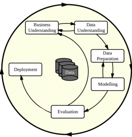
Business Understanding Definition of the requirements and objectives of a data mining project from the business (or domain) perspective. In-situ exploration techniques attempt to overcome this problem by allowing direct examination of the data files [Idr11].

Objectives

Structure of this document

Chapter 7 discusses our contribution and analyzes the threats to the validity of the present thesis. Participants The direct participants in the current research are the researcher, the supervisors and the thesis supervisors.

Research strategy

A systematic mapping study is a procedure for investigating the situation of a broad research area with a high degree of granularity, which allows us to identify parts of the domain that may be interesting to investigate in more detail [KC07]. For completeness, we have included in Figure 2.2 a process diagram for a systematic mapping study as defined by Petersen et al.

Data generation methods

Upgrade and improve Embodiment design Conceptual design Clarification of the task Detail design Optimizing the layout and forms Optimizing the principle.

Data analysis

Open Science

We summarize in this chapter the stages and results of the systematic mapping of the literature, a process described in Section 2.1. Because the Engineering Design Process is iterative and includes feedback loops, we present the objectives of the original literature mapping in Section 3.1.

Method

• Research questions
• Search strategy
• Study selection criteria
• Classification
• Data extraction and visualization

A set of known works taken from [IPC15] because our RQ2 is not covered by the original classification. To answer our second research question - the maturity of the area - we follow the classification of research approaches made by [Wie06], as do our guidelines for systematic design [Pet07].

Results

Study selection

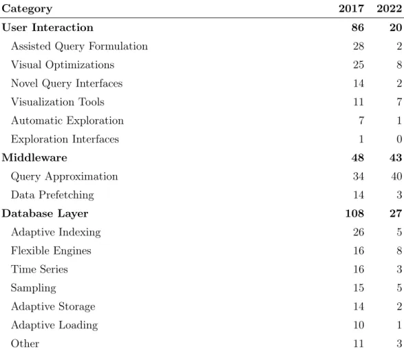
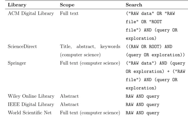
Note that only the ACM Digital Library was queried for the 2022 end-of-year update, as it indexes the most important journals and conferences from 2017 — see Table 3.6. For the ACM Digital Library search, we specifically filtered out non-primary studies, although some were still found.

Study data extraction

International Conference on Extending Database Technology 3 International Workshop on Data Management on New Hardware 3 ACM SIGMOD Symposium on Principles of Database Systems 2. IEEE International Conference on Mobile Data Management 2 Intelligent Information Systems and Database Systems 2 International Conference on Advanced Cloud and big data 2.

Discussion

Answering the research questions

We can see that there is one study that covers the three requirements: A distributed in situ analysis method for large-scale scientific data, D. Hanet al. Although they mention access to the raw files and the fact that it is distributed, they do not explicitly state anything about their interactivity.

Study insights

Threats to validity

Discussion of relevant methods

• All three requirements
• Distributed access to raw files
• Interactive access to raw files
• Distributed and interactive
• Summary

While other tools track the provenance of the data at the file level and leave it up to the user to compare the records. The user must provide a description of the data schema, which FlashView uses to sample the file when the first query comes in.

Conclusions

Known events / known algorithms Use physical models to locate known phenomena of interest spatially or temporally in a large database. Unknown Events / Known Algorithms Use predictive models to predict the presence of unseen events in a large and complex database. In Section 4.1, we use an existing astronomy database to expand our understanding of how users explore datasets.

Refining objectives

Solution principles

• n-IND finding algorithms
• Foreign Key Discovery
• Complementarity
• Schema Homogenization

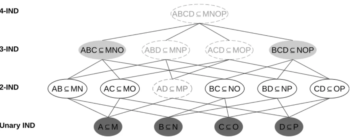
This partial order allows us to structure the search space as a grid, as illustrated in figure 4.2. Most solutions make use of this property to explore the search space in a bottom-up —from levelk tok+1— or top-down —from levelk to k–1— order. While these three algorithms have been evaluated on IND between relational datasets and with attributes that can be compared directly (i.e., from discrete domains), their traversal of the search space and their validation steps are well decoupled.

Proposed solution

Equally Distributed Dependencies

Instead, we can use R.X =d S.Y as an approximation, which means that the two sets of attributes are evenly distributed. With these rules we have defined the search space similar to that of IND Discovery. Example 2 If we have two sets of 10 attributes that are equally distributed, the number of three-dimensional projections (specializations) that must be equally distributed will be 103.

Uniform n-Hypergraphs and quasi-cliques

DEFINITIONS This property is similar to that proposed forINDs[DLP02], with the exception that even if d |= I2, there is a probability of falsely rejecting I1, bound by the significance levelα. If we have a significance level of α = 0.1, then the expected number of falsely rejected 3-dimensional equalities is 12.

Inferring common multidimensional data

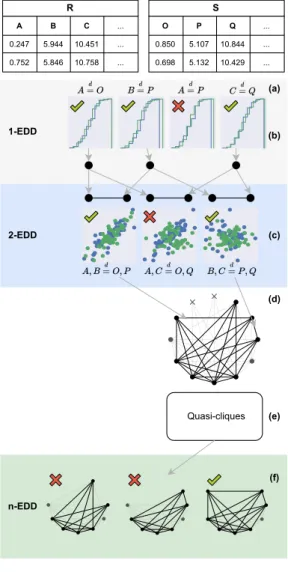
Uni-dimensional EDDs

We propose to use an interval tree constructed over the entire dataset to reduce the number of tests. Building the tree can be done in O(Nlog(N)) time, and each search can be done inO(log(N) +m), where 'm is the number of overlapping intervals for a given attribute. However, the cost of the tests themselves is virtually negligible compared to the cost of finding n-ary EDDs, which is exponential with the number of unary EDDs.

Multidimensional EDDs

Given this initial hypergraph, the authors of Find2 prove that finding the highest arityINDs can be compared to the problem of finding cliques, since all generalized k-ary INDs must appear as edges. Cliques are likely to be broken due to false rejections and there will be false edges due to false positives. Any rejected EDD is added to the negative limit and will not be considered again.

PresQ algorithm

If Find2 finds high-arity EDDs, it is because Hyperclique finds maximum cliques close to the maximum quasi-clique. Growing the quasi-cliques: This is similar to the idea of ​​KernelQC [SDT18], but based on a quasi-clique enumeration algorithm. In other words, if the degree of a node within a quasi-clique candidate is less than the critical value, we can reject the null hypothesis and accept that the set of edges connecting the node are spurious.

Experiments

Experimental design

This experiment measures, in a controlled way, the ability of the algorithms to find the true clique and how their running time is affected by the number of missing and false edges. However, regardless of the test chosen, there will always be a number of false negatives related to the level of significance. Given the variability and number of dimensions, it can be difficult to assess the quality of the results.

Environment

Results

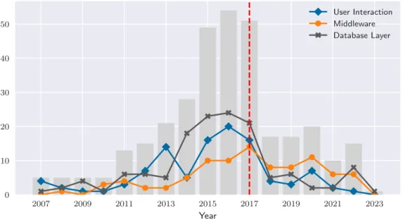
Influence of spurious edges: We show in Figure 5.3 the performance of the algorithms for 3-hypergraphs and different proportions of spurious edges. Interestingly, there is an inverse correlation between the number of missing edges and the running time. The number of 1-EDDs increases steadily as relationships are added, but 2- and n-EDDs remain relatively stable (the corresponding error bars overlap), and so does the running time.

Conclusions

While a formal statistical test may be more appropriate when the alternative hypothesis is known, machine learning classifiers may be a good alternative when the data is complex and abundant [Kir20;Kim21; Liu20]. Furthermore, the representation "learned" by some classifiers can be useful for investigating how the samples differ [Fri03;LU17], or it can be used later for other purposes, such as directly classifying future samples. The learned map can be directly used for unsupervised clustering and classification tasks if the training data is labeled [UM05;Ult07].

Definitions

The output space is modeled as a grid of neurons – a neural map – that responds to a set of values ​​from the input space [Koh82]. The output model preserves the topology of the input space: every continuous change in the input data causes a continuous change on the neural map [Vil99]. Each neuron i from the model has an associated weight vector with the same dimensionality as the input space,wi(t), corresponding to the epoch of the training phase.

The intuition behind this is that if two samples are equally distributed in the input space, they should also be equally distributed in the output space. We calculate how many points of X and how many of Z are assigned to a given neuron. Finally, we perform a two-sample aχ2 test, comparing the counts for both samples on the output space.

Experimental setup

Evaluated alternatives

EXPERIMENTAL SETUPS with any test based on binning, its major drawbacks are that its results. Kernel methods are based on calculating the maximum mean discrepancy (MMD) between the samples, which is the distance between their expected functions in a reproducing kernel Hilbert space.

Results

• Normal distribution
• DC2 Dataset
• Open University Learning Analytics Dataset
• Eye Movements Dataset
• Age (IMDb Faces) Dataset
• PresQ results

We take all students from the lower end of the poverty line and a sample of equal size from the general population to test this hypothesis. If we select one of the cells with the greatest bias towards low-income students, we can see that it only contains young female students from the Northwest region. During classification, objects can be labeled according to the label of the neuron into which they are mapped.

Conclusions

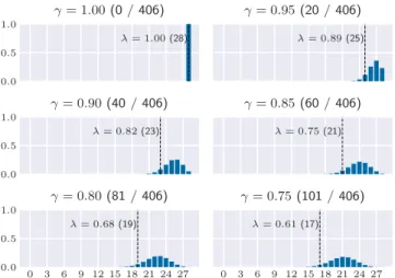
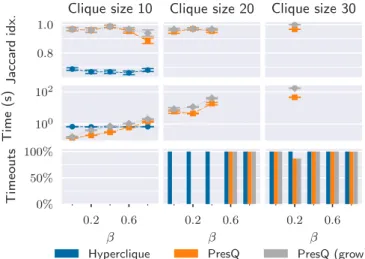
The results from the quasi-clique test set (section 5.3.3) show that the initial phase of PresQ produces results close to the original cliques on uniform n-hypergraphs. Instead, we propose an intuitive and statistically interpretable method to dynamically adjust the threshold to the extent that it is expected to follow a hypergeometric distribution and which can be adjusted based on the quasi-clique itself, as shown in Equation 5.8. This is due to traversing the search space and validating the EDDs represented by the quasi-cliques.

Two-sample test based on Self-Organizing Map

Threats to validity

Internal validity

The search algorithm based on VALIDITY THREATS consistently performs better in terms of both runtime and ability to find the maximum EDD. However, we consider that the runtime differences are significant enough to make quasi-clique-based search a better approach in those cases. Since the relative changes will remain similar, we are sure that the benefits come from the algorithm and not from its implementation.

External validity

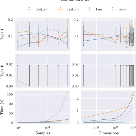
For the proposed two-sample statistical test, the results in section 6.5 come from running the tests between 200 and 2000 times, with independent randomized samples. Similarly, the experiments for the SOM-based two-sample statistical test were conducted over five different datasets and compared with kernel-based and machine learning-based alternatives. Finally, in Section 8.3 we propose possible future lines of work to improve or build on the contributions from the current work.

Contributions

• Survey of state of the art
• New category for Interactive Data Exploration
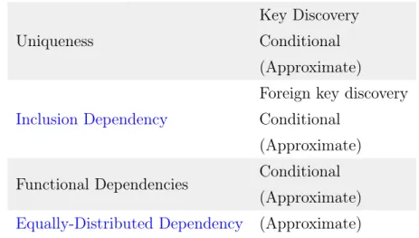
• Definition of Equally-Distributed Dependency
• Algorithms
• Publications
• Software

At the end of 2022, we updated our study to check the development of the research. The results of this study, presented in Chapter 3, are a valuable state-of-the-art update and contribute to the first subgoal: to find existing techniques that help users explore the data in-situ. One could argue that the logical file containing a given subset of the data is a detail that can be integrated into an existing index.

Future work

Where are my results?” In: CIDR ’11: Fifth Biennial Conference on Innovative Data Systems Research (2011), pp. Clarity bordering on stupidity': where's the quality in systematic review?" In:Journal of Education Policy pp. A Machine Learning Approach to Foreign Key Discovery." In: 12th International Workshop on the Web and Databases.

Benchmarking Equally-Distributed Dependency finding

Find2 vs. PresQ

Scalability

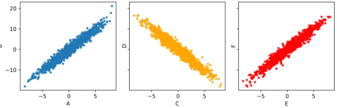
In this appendix, we briefly describe an insight and two prototypes generated during the development of this thesis that did not prove successful. This is possible under the assumption that there are three types of correlations or dependencies:

File Correlation

Since trees are a commonly used data structure for spatial partitioning - KD-Tree, Binary Partition Tree, R-Tree - we trained two decision trees on both catalogs using sky coordinates as features.

Offset Correlation

Attribute Correlation