Open problems on reachability and exact controllability for the heat equation
Marius Tucsnack
Institut de Math´ematiques de Bordeaux
August 19, 2019
This talk presents open problems on reachability and exact controllability for the heat equation.
1
From the reachable space of the heat equation to Hilbert spaces of holomorphic functions
Andreas Hartmann∗, Karim Kellay†, Marius Tucsnak‡ July 27, 2017
Abstract
This work considers systems described by the heat equation on the interval [0, π] with L2 boundary controls and it studies the reachable space at some instant τ > 0. The main results assert that this space is generally sandwiched between two Hilbert spaces of holomorphic functions defined on a square in the complex plane and which has [0, π] as one of the diagonals. More precisely, in the case Dirichlet boundary controls acting at both ends we prove that the reachable space contains the Smirnov space and it is contained in the Bergman space associated to the above mentioned square. The methodology, quite different of the one employed in previous literature, is a direct one. We first represent the input-to-state map as an integral operator whose kernel is a sum of Gaussians and then we study the range of this operator by combining the theory of Riesz bases for Smirnov spaces in polygons and the theory developed by Aikawa, Hayashi and Saitoh on the range of integral transforms, in particular those associated with the heat kernel.
1 Introduction We consider the system
∂w
∂t(t, x) = ∂2w
∂x2(t, x) t>0, x∈(0, π), w(t,0) =u0(t), w(t, π) =uπ(t) t∈[0,∞),
w(0, x) = 0 x∈(0, π),
(1.1)
which models the heat propagation in a rod of lengthπ, controlled by prescribing the temper- ature at both ends. It is well known (see, for instance, [9, Proposition 10.7.3]) that for every u0, uπ ∈ L2[0,∞) the problem (1.1) admits a unique solution w ∈ C([0,∞), W−1,2(0, π)).
(Recall that W−1,2(0, π) is the dual of the usual Sobolev space W1,2(0, π) with respect to
∗Institut de Math´ematiques de Bordeaux, Universit´e de Bordeaux/Bordeaux INP/CNRS , 351 Cours de la Lib´eration, 33 405 TALENCE, France, [email protected]
†Institut de Math´ematiques de Bordeaux, Universit´e de Bordeaux/Bordeaux INP/CNRS, 351 Cours de la Lib´eration, 33 405 TALENCE, France, [email protected]
‡Institut de Math´ematiques de Bordeaux UMR 5251, Universit´e de Bordeaux/Bordeaux INP/CNRS, 351 Cours de la Lib´eration, 33 405 TALENCE, France, [email protected]
the pivot spaceL2[0, π].) Moreover, according to the same reference, theinput-to-state maps (Φτ)τ >0 defined by
Φτ [u0
uπ ]
=w(τ,·) (τ >0, u0, uπ ∈L2[0, τ]), (1.2) lie, for every τ > 0, in L(L2([0, τ];U), W−1,2(0, π)). In control theoretic terms, this means that (1.1) defines a well-posed control system, with state space X =W−1,2(0, π) and input space U =C2. A classical important question in the study of control systems consists in the characterization of theirreachable spaceat instantτ, which is the space of states which can be attained at instantτ when the input is freely moving inL2([0, τ];U). In our case this space is the range of Φτ, denoted Ran Φτ, where Φτ has been defined in (1.2). As far as we know, the first results on this space for the boundary controlled heat equation have been given in the classical paper of Fattorini and Russell [4], where it is shown that the functions which can be extended to holomorphic ones in a horizontal strip containing [0, π] and which vanish, together with all their derivatives of even order, at x= 0 and x=π, belong to Ran Φτ. This result implies, in particular, that Ran Φτ ⊃RanTτ, whereT is the semigroup generated by the 1DDirichlet Laplacian in W−1,2(0, π), which means that the system determined by (1.1) is null-controllable in any timeτ >0. As remarked in Seidman [8] this means, in particular, that Ran Φτ is invariant with respect toτ >0.
The first significant improvement of Fattorini’s and Russell’s result on this reachable space has been reported only in 2016, in the work by Martin, Rosier and Rouchon [7], where it has been shown that any function which can be extended to a function holomorphic in a certain disk inCcontaining the segment [0, π] lies in the reachable space. This result has been further improved in Dard´e and Ervedoza [2], where it has been shown that any function which can be extended to one which is holomorphic in a neighbourhood of the squareD defined by
D={s=x+iy∈C | |y|< x and |y|< π−x}, (1.3) lies in the reachable space.
On the other hand, it is not difficult to check (see, for instance, [7, Theorem 1]) that if ψ∈Ran Φτ thenψcan be extended to a function holomorphic inD, so that the assertion in [2] looks almost sharp. The aim of our work is to show that this result can be significantly improved, by showing that Ran Φτ can be sandwiched between two Hilbert spaces of analytic functions defined onD. The methodology we employ, completely different of those used in [7]
or [2], is based on explicit series form representations of the solutions of (1.1), combined with results on Bergman and Smirnov spaces on D. For the sake of completeness, we recall the definitions of the above mentioned spaces. First, given an open set Ω⊂C, theBergman space A2(Ω) consists of all functions holomorphic in Ω with ∫
Ω|f(x+iy)|2dxdy < ∞. Endowed with the norm induced fromL2(Ω),A2(Ω) is clearly a Hilbert space. We will also use weighted Bergman spaces. Let ω be a positive measurable function on Ω, then A2(Ω, ω) is the space of holomorphic functions for which∫
Ω|f(x+iy)|2ω(x+iy) dxdy < ∞. The Smirnov space on a simply connected domain Ω can be defined provided that there is a conformal map φ from the unit diskD to Ω. If Γr is the image under φ of the circle |z|=r, then f ∈E2(Ω) if and only if supr<1∫
Γr|f(z)|2|dz|<∞. The curves Γr can be replaced by any sequence of rectifiable Jordan curves surrounding eventually every compact subdomain of Ω (see Duren [3]). If Ω is a Smirnov domain (in particular a polygon like D, see [5, Ch.VII,Thm. 4.6])
then, according to [3, p. 184]) we have thatf ∈E2(Ω) ifff ∈L2(∂Ω) with
∫
∂Ω
ζnf(ζ) dζ = 0 (n∈N).
In this case, the norm inE2(Ω) is given by
∥f∥2E2(Ω)=
∫
∂Ω
|f(ζ)|2|dζ|.
With the above definitions, the result in [7], asserting that Ran Φτ ⊂ Hol (D) (the space formed by the functions holomorphic onD), can be strengthened to
Proposition 1.1. For every τ >0 we have Ran Φτ ⊂A2(D).
Our main result improves the existing lower bounds of the reachable space and states as follows:
Theorem 1.2. For every τ >0 we have Ran Φτ ⊃E2(D).
Remark 1.3. It turns out that the inclusion in Theorem 1.2 is strict (see Proposition 4.3 below). We do not have a similar result for the inclusion in Proposition 1.1. In view of the methodology used below, we conjecture that we haveRan Φτ =A2(D).
The paper is organized as follows. In the next section we prove Proposition 1.1 using a series representation, based on the 1D heat equation kernel, of the input-to-state map. As it turns out below, the domain of holomorphy and the behavior of the sum of this series near the boundary of the holomorphy domain are determined by a dominating term, which is treated using a result by Aikawa, Hayashi and Saitoh on Laplace-type transforms having their range in Bergman spaces. In Section 3, following work by Levin-Lyubarskii, we introduce a Riesz basis of exponentials in the Smirnov spaceE2(D) which allows us to decompose functions in E2(D) into a sum of two functions in Bergman spaces associated with two infinite sectors. In Section 4 this allows us, in particular, to decompose functions in the Smirnov spaceE2(D) into a dominating term for which we use again Aikawa, Hayashi and Saitoh, and remainder terms which are “small” in appropriate weighted Bergman spaces on infinite sectors. Using a matrix type argument, this allows us to prove Theorem 1.2. In the last section we discuss the adaptations of our methods and results to some other boundary conditions and controls.
2 Proof of Proposition 1.1
Using the decomposition of the solutionwof (1.1) in the standard Fourier basis (sin(nx))n>1
of L2[0, π], it is not difficult to check that the input to state maps (Φτ)τ>0 defined in (1.2) write
(Φτu)(x) =∑
n>1
n [∫ τ
0
en2(σ−τ)u0(σ) dσ ]
sin(nx)
+∑
n>1
n(−1)n+1 [∫ τ
0
en2(σ−τ)uπ(σ) dσ ]
sin(nx) (τ >0, x∈(0, π)),
where the above series converges in W−1,2(0, π), uniformly with respect to σ ∈[0, τ]. From the last formula it follows that
(Φτu)(x) =
∫ τ
0
∂K0
∂x (τ −σ, x)u0(σ) dσ+
∫ τ
0
∂Kπ
∂x (τ −σ, x)uπ(σ) dσ (x∈[0, π]), (2.4) where
K0(σ, x) =−∑
n>1
e−n2σcos(nx)
=−1 2
∑
n>1
e−n2σ(
einx+ e−inx)
=−1 2
∑
n∈Z
e−n2σeinx (σ >0, x∈(0, π)). (2.5) Kπ(σ, x) =−K0(σ, π−x) (σ >0, x∈(0, π)). (2.6) We note that forσ >0 we can extend K0(σ,·) andKπ(σ,·) to functions inL2loc(R) of period 2π. Formulas (2.5) and (2.6) have been widely used, often combined with duality arguments, to study the controllability properties of the system (1.1). However, it seems that this way of writing the kernels K0 and Kπ is not very useful to prove reachability results beyond those classically obtained in [7]. We thus use an alternative form of K0 and Kπ, in terms of the heat kernel on the real line. For the sake of completeness, we derive below these formulae using the Poisson summation formula. Alternatively, these expressions ofK0andKπ could be obtained using the classical method of images, which allows deriving fundamental solutions of linear partial differential equations on a segment with appropriate boundary conditions from the corresponding fundamental solution for the same PDE on the whole line.
Proposition 2.1. We have K0(σ, x) =−1
2
√π σ
∑
m∈Z
e−(x+2mπ)24σ (σ >0, x∈R), (2.7)
Kπ(σ, x) = 1 2
√π σ
∑
m∈Z
e−(x+(2m−1)π)2
4σ (σ >0, x∈R), (2.8)
where the above series converge in L2[0, π].
Proof. We first remind the formula of the Fourier transform of a Gaussian, given by Gbα =
√π αG1
4α (α >0), (2.9)
where
Gα(y) = e−αy2 (y ∈R).
For a > 0, γ0 = 2πa and f ∈ S(R), we also remind the Poisson summation formula in the
form ∑
m∈Z
f(x+ma) = 1 a
∑
k∈Z
fˆ(kγ0)eikγ0x (x∈R). (2.10)
We first apply (2.10) withf(y) = e−y
2
4σ and a= 2π, so that γ0 = 1. Since, according to (2.9), we have
fˆ(ξ) =√
2πσe−σξ2 (ξ ∈R),
we obtain √
√π σ
∑
m∈Z
e−(x+2mπ)24σ =∑
n∈Z
e−σn2einx (x∈R).
The above formula and (2.5) imply (2.7).
Finally, (2.8) follows from (2.7) and the fact thatKπ(σ, x) =−K0(σ, π−x).
Our strategy to study Ran Φτ is to identify in each of the formulae forK0 andKπ in (2.7) and (2.8) a principal term which corresponds, roughly speaking, to a boundary controlled heat equation on a half-line, and to show that the remaining terms can be seen as perturbations.
To determine the range of the operators corresponding to the principal parts we use in an essential manner the following result from Aikawa, Hayashi and Saitoh [1].
Theorem 2.2. Let
∆ ={s∈C | −π
4 <args < π 4}. Fors∈∆, τ >0 and f ∈L2[0, τ]we set
(Pτf)(s) =
∫ τ
0
se−
s2 4(τ−σ)
2√
π(τ−σ)32 f(σ)√
σdσ. (2.11)
ThenPτ defines an isometric isomorphism from L2[0, τ]onto A2(∆, ω0), where ω0(s) = eRes
2 2τ
τ (s∈∆). (2.12)
A simple change of variables gives the following consequence of the above theorem.
Corollary 2.3. With the notation in Theorem 2.2, let
∆ =˜ π−∆.
Fors∈∆,˜ τ >0 and f ∈L2[0, τ]we set
(Qτf)(s) =
∫ τ
0
(π−s)e−
(π−s)2 4(τ−σ)
2√
π(τ−σ)32 f(σ)√
σdσ. (2.13)
ThenQτ defines an isometric isomorphism fromL2[0, τ]onto A2( ˜∆, ωπ), where ωπ(s) = eRe(π2τ−s)2
τ (s∈π−∆). (2.14)
Remark 2.4. The operators Pτ ans Qτ defined above are closely related to the derivative with respect to x of the terms corresponding to m = 0 in the definition (2.7) of K0 and in the definition (2.8) of Kπ, respectively. Alternatively, these operators can be connected to the heat equation on a half-line. More precisely, setting
wl(t, x) = (Ptf)(x) (t>0, x>0),
we have that
∂wl
∂t (t, x) = ∂2wl
∂x2 (t, x) (t>0, x>0), wl(t,0) =√
tf(t), t∈[0,∞),
wl(0, x) = 0 x>0,
.
Similarly, setting
wr(t, x) = (Qtf)(x) (t>0, x6π),
we have that
∂wr
∂t (t, x) = ∂2wr
∂x2 (t, x) (t>0, x 6π), wr(t, π) =√
tf(t), t∈[0,∞),
wr(0, x) = 0 x>0,
.
The presence of the factor √
t in the boundary conditions above (and consequently in the definition of Pτ and Qτ) is important in order to use the results in [1], where this factor allows using the explicit form of the reproducing kernel ofA2(∆).
We next give a simple lemma to be used in the proof of Theorem 1.1.
Lemma 2.5. Let τ >0 and u∈L2[0, τ] and denote φτ(s) =
∫ τ
0
e− s
2 4(τ−σ)
(τ −σ)3/2su(σ) dσ (s∈D).
Thenφτ ∈A2(D) and there exists a positive constantCτ such that
∥φτ∥A2(D)6Cτ∥u∥L2[0,τ] (u∈L2[0, τ]).
Proof. We first write φτ =φτ,1+φτ,2, where φτ,1(s) =
∫ τ
2
0
e− s
2 4(τ−σ)
(τ−σ)3/2su(σ) dσ (s∈D), φτ,2(s) =
∫ τ
τ 2
e−
s2 4(τ−σ)
(τ −σ)3/2su(σ) dσ (s∈D).
It is easy to check that
∥φτ,1∥A2(D)6C˜τ∥u∥L2[0,τ] (u∈L2[0, τ]),
for some positive constant ˜Cτ. We thus only have to estimate the norm ofφτ,2 inA2(D). To this aim we define the following function on [0, τ] by
˜ u(t) :=
0 if t∈[0, τ /2], u(t)√
t if t∈[τ /2, τ].
Using Theorem 2.2, we get
∥φτ,2∥2A2(D) = 4π∥Pτu˜∥2A2(D) 6 4πτ∥Pτu∥˜ 2A2(∆, ω0)
= 4πτ∥u˜∥2L2[0,τ]
= 4πτ
∫ τ
τ /2
|u(σ)|2 σ dσ 6 8π∥u∥2L2[0,τ].
We are now in a position to give the main proof in this section.
Proof of Proposition 1.1. Let K˜0(σ, s) =−1
2
√π σ
∑
m∈Z∗
e−(s+2mπ)24σ (σ >0, s∈D), (2.15)
and
K˜π(σ, s) = 1 2
√π σ
∑
m∈Z∗
e−(s+(2m−1)π)2
4σ (σ >0, s∈D). (2.16)
Let ψ(x) =˜
∫ τ
0
∂K˜0
∂x (τ −σ, x)u0(σ) dσ+
∫ τ
0
∂K˜π
∂x (σ, x)uπ(σ) dσ (x∈[0, π]). (2.17) By Lemma 2.5 it suffices to prove that ˜ψcan be extended to a function holomorphic inA2(D).
To this aim, we note that there existsa, b >0 such that for everyk∈Z\ {−1,0} we have (s+kπ)e−
(s+kπ)2
4(τ−σ)26ak2e−
bk2
(τ−σ) (s∈D).
It follows that for everys∈D and for everyk∈Z\ {−1,0}we have
∫ τ
0
(s+kπ)e−
(s+kπ)2 4(τ−σ) 2
(τ −σ)3 dσ 6a
∫ τ
0
k2e−bk
2 t
t3 dt= a b2k2
∫ ∞
bk2 τ
ue−udu6C (1
τ + 1 )
e−bk
2 τ . The fact that ˜ψ is in A2(D) follows by combining the last estimate with the use of the Cauchy-Schwarz inequality in (2.17). This achieves the proof.
3 A decomposition result in E2(D)
The aim of this section is to show that functions inE2(D) can be decomposed into a sum of two functions each of which being in a weighted Bergman space defined on an unbounded sector.
An important ingredient in deriving this decomposition is a Riesz basis of exponentials in the Smirnov classE2(D), which is constructed using results from B. J. Levin and J. I. Ljubarski˘ı
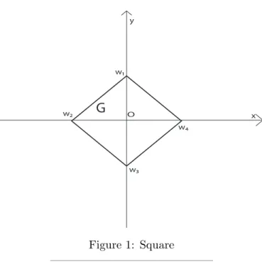
G
Ox y
w1
w2
w3
w4
Figure 1: Square
——————————————
[6]. To apply some of these results it is more convenient to replaceDby a square containing the origin. Denote
D˜ =−π
2 +D. (3.1)
To apply results from [6] we need some notation. Let w1 = π
2i, w2 =−π
2, w3 =−π
2i, w4 = π
2, (3.2)
be the vertices of the square ˜D(see Figure 1).
For j ∈ {2,3,4} we denote by lj the edge joining wj−1 and wj, whereas l1 is the edge joiningw4 to w1. We also denote by θj the angle formed by the exterior normal to lj with the positive sense of theOx axis, so that
θ1 = π
4, θ2 = 3π
4 , θ3 = 5π
4 , θ4 = 7π
4 . (3.3)
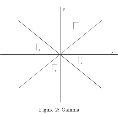
We also define (see Figure 2) the sectors
Γj ={λ∈C | argλ∈(θj, θj+1)}.
Consider theangular support function of ˜D defined by H(λ) = Re(wjλ) for λ∈Γj. We thus have
H(λ) =1 2
πImλ forλ∈Γ1,
−πReλ forλ∈Γ2,
−πImλ forλ∈Γ3, πReλ forλ∈Γ4.
(3.4)
Forj∈ {1,2,3,4} and K >0 we set Πj(K) =
{
λ∈C | Re(λe−iθj)>0, Im(λe−iθj)< K }
.
x x y
1
2
3
4
Figure 2: Gamma
——————————————
Finally, for everyK >0 we introduce
D˜K=∪4j=1Πj(K).
The above notation has been used in [6] to introduce a class of functions playing an important role in the construction of Riesz bases of exponentials in Smirnov spaces defined on general convex polygons containing the origin. For the sake of simplicity, we recall below some definitions and results from [6] when the polygon is chosen to be the above defined square ˜D.
Definition 3.1. The class of functionsSD˜ is formed by the functionsSwhich are holomorphic onD, of exponential type and˜
1. The functionS has a sequence (λk)k∈Z of simple zeros and there existsK >0 such that all these zeros lie in D˜K;
2. infj̸=k|λj−λk|= 2δ >0;
3. There exist c, C >0 such that
0< c <|S(λ)|e−H(λ)< C (λ̸∈D˜K).
Theorem 3.2. With the notation in Definition 3.1, the family (
eλkze−H(λk))
k∈Z is a Riesz basis in E2( ˜D).
With the change of variable behind (3.1) in mind, we obtain the following consequence of Theorem 3.2:
Corollary 3.3. With the above notation, the family ( gλ)
λ∈Λ defined by
gλ(s) = eλse−λπ2 e−H(λ) (λ∈Λ, s∈C), (3.5) is a Riesz basis inE2(D).
With the indicator function of ˜Dgiven by (3.4), as asserted in [6], a functionS satisfying the conditions in Definition 3.1 is
S(λ) =
∑4 j=1
ewjλ (λ∈C), (3.6)
wherewj are defined in (3.2). More precisely, we have S(λ) = eπ2λ+ e−π2λ+ eiπ2λ+ e−iπ2λ
= 2 cos (π
2λ )
+ 2 cos (
iπ 2λ
)
= 4 cos
(π(1 +i)λ 4
) cos
(π(1−i)λ 4
)
(λ∈C).
The zeros ofS form the set Λ defined by
Λ ={(2k+ 1)(1±i) :k∈Z}. (3.7)
We next use the Riesz basis constructed above to show that functions inE2(D) can be written as sum of two functions, each of which is in a Bergman space defined on an infinite sector.
To this aim, let
∆ = {
s∈C | −π
4 <args < π 4
}
. (3.8)
Lemma 3.4. Let Λ be the sequence introduced in (3.7) and let the polynomial function p be defined by
p(s) =s+ 2πi (s∈C). (3.9)
Let φ∈E2(D) with φ=∑
λ∈Λaλgλ. Denote φ1 = ∑
λ∈Λ Reλ<0
aλgλ and φ2 = ∑
λ∈Λ Reλ>0
aλgλ.
Thenφ1/p∈A2(∆) et φ2/p∈A2(π−∆).
Proof. We first note that using (3.4) it follows that
|e−(2k+1)(12 ±i)πe−H((2k+1)(1±i))|= 1 (k6−1). (3.10) Moreover, for everyk6−1 andx+iy∈∆ we have
|e(2k+1)(1+i)(x+iy)|= e(2k+1)(x−y), |e(2k+1)(1−i)(x+iy)|= e(2k+1)(x+y), so that
|eλ(x+iy)|6e(Reλ)(x−|y|) (x+iy∈∆, λ∈Λ, Reλ <0). (3.11) We also note that there existsc >0 such that
|p(x+iy)|2> 1
2(x2+c) (x+iy∈∆). (3.12)
Indeed|p(x+iy)|2−12x2= 12x2+ (y+ 2π)2 is vanishing only in the point (0,−2π), which is far away from ∆∪(π−∆), so that on this set it is bounded from below by a strictly positive
constant. Combining (3.12) and (3.11) it follows that for every λ, µ∈Λ with Reλ <0 and Reµ <0 we have:
⟨gλ p ,gµ
p
⟩
A2(∆)
6
∫
∆
eλs |eµs|
|p(s)|2 dxdy 6
∫
∆
e(x−|y|)(Reλ+Reµ)
|p(x+iy)|2 dxdy
6 4
∫ +∞
0
ex(Reλ+Reµ) x2+c
( ∫ x
0
ey(−Reλ−Reµ)dy )
dx
= 4
−Reλ−Reµ
∫ +∞
0
ex(Reλ+Reµ)(
ex(−Reλ−Reµ)−1)
x2+c dx
6 4
−Reλ−Reµ
∫ +∞
0
dx x2+c
6 C 1
(|Reλ|+|Reµ|),
for a suitable constantC. Using Hilbert’s inequality it follows that φ1
p 2
A2(∆)
= ∑
λ,µ∈Λ Reλ<0 Reµ<0
aλaµ
⟨gλ p ,gµ
p
⟩
A2(∆)
6 C
2
∑
λ,µ∈Λ Reλ<0 Reµ<0
|aλ||aµ|
|Reλ|+|Reµ|
6 Cπ
2
∑
λ∈Λ Reλ<0
|aλ|2,
which shows thatφ1/p∈A2(∆).
To prove that φ2/p∈A2(π−∆), let λ∈Λ, with Reλ >0 and remark that gλ(π−s) =g−λ(s) (s∈∆).
Denotingq(s) :=p(π−s), we have
|q(x+iy)|2=|p(π−s)|2 = (π−x)2+ (y−2π)2> 1
10(x2+d) (x+iy∈∆), for a suitably chosend >0. Indeed, arguing similarly as above we have
|π−s+ 2π|2− 1
10x2 = 9 10
( x−10
9 π )2
+ (y−2π)2− 1
9π2 (x+iy∈∆).
The right-hand side of the above equality vanishes on an ellipse which stays strictly away from
∆ and hence it admits a strictly positive minimum there. Consequently, for everyλ, µ∈Λ,
with Reλ, Reµ >0 we have
⟨gλ p ,gµ
p
⟩
A2(π−∆)
=
⟨g−λ q ,g−µ
q
⟩
A2(∆)
6
∫
∆
e(x−|y|)(−Reλ−Reµ)
|q(x+iy)|2 dxdy
6 20
∫ +∞
0
ex(−Reλ−Reµ) x2+d
( ∫ x
0
ey(Reλ+Reµ)dy )
dx
6 C
Reλ+ Reµ,
whereC is a constant possibly different from the preceding case. Using, as above, Hilbert’s inequality, we conclude thatφ2/p∈A2(π−∆), which ends the proof.
At this point we recall, given an open set Ω ⊂ C, the classical notation H∞(Ω), which stands for the space of bounded analytic functions in Ω.
Lemma 3.5. Let η >0 and letp be defined by (3.9). Then there existsf ∈Hol(∆∪(π−∆)) satisfying the following conditions
(i) p(s)eηs2
f(s) ∈H∞(∆), (ii) p(s)eη(π−s)2
f(s) ∈H∞(π−∆).
Proof. We first note that if suffices to construct a functiong such that (i’) 1
g(s) ∈H∞(∆) (ii’) e−2πηs
g(s) ∈H∞(π−∆)
Indeed, assuming the existence ofgwith the above properties, we see thatf(s) = eηs2g(s)p(s) satisfies the requirements in the conclusion of the lemma.
We show below that the function g defined by g(s) = cosh(cs)
r(s) (s∈∆∪(π−∆)),
where c > 2πη and r is an appropriately chosen polynomial, satisfies the above conditions.
More precisely, letr be defined by r(s) = ∏
µ∈I
(s−µ) (s∈C), where
I = {
−i c(n+1
2)π) }
n∈Z∩[−iπ, iπ].
Note that I is the set formed by the roots of cosh(cs) on the segment [−iπ, iπ]. Clearly, g∈Hol(∆∪(π−∆)) and 1/g∈Hol(∆∪(π−∆)).
We still have to show thatg satisfies conditions (i’) and (ii’) above. To this aim, it clearly suffices to show that
|g(s)|>Const e2πη|x|, s=x+iy∈∆∪(π−∆). (3.13) To check the above estimate, lets=x+iy∈∆∪(π−∆), with|x|> 1c. Then
|cosh(cs)|2 = 1
22ec(x+iy)+ e−c(x+iy)2= 1 4
(e2cx+ e−2cx+ 2 cos(2y))
> 1
4(e2c|x|−2), It follows that there existsC >0 such that
|cosh(cs)|>Cec|x| (s=x+iy∈∆∪(π−∆), |x|> 1 c).
Denoting byN the degree of r we have
|r(s)|6Const |s|N 6Const (1 +|x|)N, s∈∆∪(π−∆).
Hence, recalling thatc >2πη, we obtain, for s=x+iy∈∆∪(π−∆) with |x|> 1c, that
|g(s)|= |cosh(cs)|
|r(s)| >Const ec|x|
1 +|x|N >Const e2πη|x|.
Fors=x+iy∈∆∪(π−∆) with|x|6 1c,g is non-vanishing, so that, using compactness, it is bounded from below by a strictly positive constant.
We have thus proved (3.13) which, as explained above, implies the conclusion of the lemma.
Corollary 3.6. With the notation in Lemma 3.4, let τ > 0 and φ ∈ E2(D). Then there existsφ1 ∈A2(∆, ω0), φ2∈A2(π−∆, ωπ), where the weights ω0 and ωπ are those defined in (2.12)and (2.14), respectively, such that
φ(s) =φ1(s) +φ2(s) (s∈D).
Proof. Letη = 4τ1 and let f be the corresponding function constructed in Lemma 3.5. This implies that the mappings s 7→ p(s)es2
f(s) and s 7→ p(s)e(π−s)2
f(s) , with p defined in (3.9), are inH∞(∆) and H∞(π−∆), respectively. The function s7→ f(s)φ(s) clearly lies in E2(D).
According to Lemma 3.4 we havef φ=φ1,0+φ2,0, with φ1,0p ∈A2(∆) and φ2,0p ∈A2(π−∆).
Settingψk=φk,0/p, we thus get f(s)φ(s)
p(s) =ψ1(s) +ψ2(s) (s∈D), withψ1 ∈A2(∆),ψ2 ∈A2(π−∆). Defineφ1,φ2 by
φ1(s) = p(s)
f(s)ψ1(s) (s∈∆), (3.14)
φ2(s) = p(s)
f(s)ψ2(s) (s∈π−∆). (3.15)
We clearly have φ=φ1+φ2 inD. Moreover, using Lemma 3.5 (recall that we have chosen η= 1/4τ), we have that the map
s7→φ1(s)es2/4τ = p(s)es2/(4τ) f(s) ψ1(s) lies inA2(∆). Similarly, the map
s7→φ2(s)e(π−s)2/4τ = P(s)e(π−s)2/(4τ) f(s) ψ1(s) lies inA2(π−∆), which concludes the proof.
4 Proof of the main result
Let ˜K0 and ˜Kπ be the functions introduced in (2.15) and (2.16), respectively. We decompose these functions as
K˜0(σ, s) =A(σ, s) +B(σ, s), and K˜π(σ, s) =C(σ, s) +D(σ, s), where
A(σ, s) =−1 2
√π σ
∑
m>1
e−(s+2mπ)24σ and C(σ, s) = 1 2
√π σ
∑
m>1
e−(s+(2m4σ−1)π)2 B(σ, s) =−1
2
√π σ
∑
m6−1
e−(s+2mπ)24σ and D(σ, s) = 1 2
√π σ
∑
m6−1
e−(s+(2m4σ−1)π)2. Denote
RA,τu(s) =
∫ τ
0
∂A
∂s(τ −σ, s)√
σu(σ)dσ, and similarlyRB,τ,RC,τ andRD,τ.
Lemma 4.1. Let ω0 and ωπ be the weights defined in (2.12) and (2.14), respectively. There exists an absolute constant C1 >0 such that for every u∈L2[0, τ]we have
1. RA,τu∈A2(∆, ω0) and RA,τu
A2(∆,ω0)6C1
√τ(1 +τ)3 e−π2/τ
1−e−π2/τ∥u∥L2[0,τ] (τ >0).
2. RB,τu∈A2(π−∆, ωπ) and RB,τu
A2(π−∆,ωπ)6C1√
τ(1 +τ)3 e−π2/4τ
1−e−π2/2τ∥u∥L2[0,τ] (τ >0).
3. RC,τu∈A2(∆, ω0) and RC,τu
A2(∆,ω0)6C1√
τ(1 +τ)3 e−π2/4τ
1−e−π2/2τ∥u∥L2[0,τ] (τ >0).
4. RD,τu∈A2(π−∆, ωπ) and RD,τu
A2(π−∆,ωπ)6C1√
τ(1 +τ)3 e−π2/τ
1−e−π2/τ∥u∥L2[0,τ] (τ >0).
Proof. Let
ρm(s, τ) =
∫ τ
0
√π
4(τ −σ)3/2(s+mπ)e−
(s+mπ)2 4(τ−σ) √
σu(σ) dσ m>1, s∈∆,
∫ τ
0
√π
4(τ −σ)3/2(s+mπ)e−
(s+mπ)2 4(τ−σ) √
σu(σ) dσ m6−1, s∈π−∆.
By the triangular and the Cauchy-Schwarz inequality we see that form>1 we have
∥ρm(·, τ)∥2A2(∆,ω0)
= 1 τ
∫∫
∆
ex
2−y2
2τ
∫ τ
0
√π
4(τ −σ)3/2(s+mπ)e−
(s+mπ)2 4(τ−σ) √
σu(σ) dσ
2 dxdy 6 π∥u∥2L2(0,τ)
16
∫∫
∆
(|x+mπ|2+y2) ex
2−y2 2τ
∫ τ
0
e−(x+mπ)2−y
2 2(τ−σ)
(τ−σ)3 dσdxdy
=
π∥u∥2L2(0,τ)
16
∫∫
∆
(|x+mπ|2+y2) ex
2−y2 2τ
∫ τ
0
e−(x+mπ)2−y
2 2σ
σ3 dσdxdy. (4.1) Setα= (x+mπ)2 2−y2. Recalling thatm>1 we see that
α= (x+mπ)2−y2
2 = x2−y2+ 2mπx+m2π2
2 > π2
2 m2 >1.
This, together with the change of variablesu=α/σ and an integration by parts, yields
∫ τ
0
e−(x+mπ)2−y
2 2σ
σ3 dσdxdy = 1 α2
∫ ∞
α/τ
ue−udu= e−α/τ
α2 (1 +α/τ) 6 e−α/τ
α (1 + 1/τ).
Using (4.1), the above estimate implies that
∥ρm(·, τ)∥2A2(∆,ω0)= 1 τ
∫∫
∆
ex
2−y2
2τ |ρm(x+iy, τ)|2dxdy
6 π
16∥u∥2L2[0,τ] (
1 +1 τ
) ∫∫
∆
ex
2−y2
2τ (x+mπ)2+y2
(x+mπ)2−y2e−x2+2mπx+m
2π2−y2
2τ dxdy.
Since|y|6x fors=x+iy∈∆ we have (x+mπ)2+y2
(x+mπ)2−y2 = 1 + 2y2
(x+mπ)2−y2 61 + 2x2
m2π2 61 +x2 (m>1, x+iy∈∆).