PDF Higgs Boson Production and Properties in the H ZZ 4 Channel

Higgs Boson Production and Properties in the

H→ZZ→4ℓ𝓁 Channel

Adish Vartak!

On behalf of the CMS Collaboration ICHEP 2014

1

H → ZZ → 4ℓ𝓁 Overview

• “Golden” channel for Higgs discovery and measurements

- High resolution and high S/B

• Statistically parched

- ~20 signal events expected with current data

- Need high lepton reconstruction, selection efficiency to catch lowest p

leptons

• We attempt to squeeze the most possible information from available events

- Exploit the rich final state topology to enhance search sensitivity and then to measure Higgs properties

- Use event-by-event mass uncertainties to measure mass

2

Event Selection

3

• Require 20/10 GeV leptons in the event (consistency with trigger)

• Lepton selection : p T > 7(5) GeV, |η| < 2.5(2.4) for e(μ), ID+isolation+IP requirements

• Construct Z candidates and recover FSR photons (ΔR<0.5)

• Select “Z 1 ” candidate with mass closest to Z peak (40 < m(Z 1 ) < 120 GeV)

• Select “Z 2 ” candidate from remaining highest p T

leptons (12 < m(Z 2 ) < 120 GeV)

• Require m(ℓ𝓁 + ℓ𝓁 - ) > 4 GeV to suppress QCD

Search Strategy (I)

• ZZ→4ℓ𝓁 events form the dominant and irreducible background

• Some additional reducible background from sources such as Z+jets, ttbar, etc.

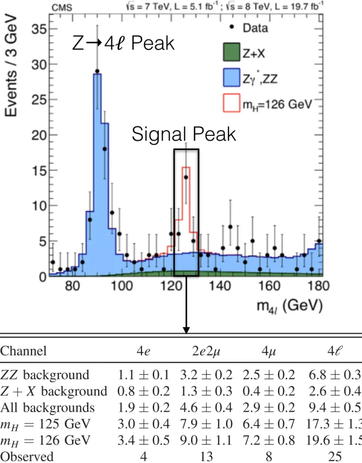
• Higgs signal produces a sharp bump on a smooth background mass

distribution

• We can see the signal peak building up around m(4ℓ𝓁) ~ 125 GeV

4

Z→4ℓ𝓁 Peak

Signal Peak

Search Strategy (I)

• ZZ→4ℓ𝓁 events form the dominant and irreducible background

• Some additional reducible background from sources such as Z+jets, ttbar, etc.

• Higgs signal produces a sharp bump on a smooth background mass

distribution

• We can see the signal peak building up around m(4ℓ𝓁) ~ 125 GeV

(m

¼ 5 126 GeV) are obtained from simulation, while the normalization and shape of the reducible background is estimated from control samples in data, as described in Sec. IX B. The error bars on data points are asymmetric Poisson uncertainties that cover the 68% probability interval around the central value [134]. A clear peak around m

¼ 126 GeV is seen, not expected from background processes, confirming with a larger data sample the results reported in Refs. [19 – 21,31]. The observed distribution is in good agreement with the expected backgrounds and a narrow resonance compatible with the SM Higgs boson with m

around 126 GeV. The Z → 4l resonance peak at m

¼ m

is observed in agreement with simulation.

The measured distribution at masses greater than 2m

is dominated by the irreducible ZZ background, where the two Z bosons are produced on shell.

The number of candidates observed in data as well as the expected yields for background and several SM Higgs boson mass hypotheses are reported in Table III, for m

> 100 GeV. The observed event rates for the various channels are compatible with SM background expectations in the m

region above 2m

, while a deviation is observed in the lower region. Given that the excess of events observed in the 4l mass spectrum is localized in a narrow region in the vicinity of 126 GeV, the events expected in a narrower range, 121.5 < m

< 130.5 GeV, are reported in Table IV . Table V reports the breakdown of the events observed in data and the expected background yields in the same m

region in the two analysis categories, together

with the expected yield for a SM Higgs boson with m

¼ 126 GeV, split by production mechanism. The m

distribution for the sum of the 4e, 2e2μ, and 4μ channels, in the mass region 70 < m

< 180 GeV, is shown in Fig. 10. Figure 11 shows the reconstructed

(GeV)

4l

m

80 100 200 300 400

Events / 3 GeV

0 5 10 15 20 25 30

35

= 126 GeV mH

*, ZZ γ Z Z+X

800 600

CMS s = 7 TeV, L = 5.1 fb^-1 ; s = 8 TeV, L = 19.7 fb^-1

FIG. 9 (color online). Distribution of the four-lepton recon- structed mass in the full mass range 70 < m

< 1000 GeV for the sum of the 4e, 2e2μ, and 4μ channels. Points with error bars represent the data, shaded histograms represent the backgrounds, and the unshaded histogram represents the signal expectation for a mass hypothesis of m

¼ 126 GeV. Signal and the ZZ background are normalized to the SM expectation; the Z þ X background to the estimation from data. The expected distributions are presented as stacked histograms. No events are observed with m

> 800 GeV.

TABLE III. The number of observed candidate events com- pared to the mean expected background and signal rates for each final state. Uncertainties include statistical and systematic sources. The results are given integrated over the full mass measurement range m

> 100 GeV and for 7 and 8 TeV data combined.

Channel 4e 2e2μ 4μ 4l

ZZ background 77 # 10 191 # 25 119 # 15 387 # 31 Z þ X background 7.4 # 1.5 11.5 # 2.9 3.6 # 1.5 22.6 # 3.6 All backgrounds 85 # 11 202 # 25 123 # 15 410 # 31 m

¼ 500 GeV 5.2 # 0.6 12.2 # 1.4 7.1 # 0.8 24.5 # 1.7 m

¼ 800 GeV 0.7 # 0.1 1.6 # 0.2 0.9 # 0.1 3.1 # 0.2

Observed 89 247 134 470

TABLE IV. The number of observed candidate events com- pared to the mean expected background and signal rates for each final state. Uncertainties include statistical and systematic sources. The results are integrated over the mass range from 121.5 to 130.5 GeV and for 7 and 8 TeV data combined.

Channel 4e 2e2μ 4μ 4l

ZZ background 1.1 # 0.1 3.2 # 0.2 2.5 # 0.2 6.8 # 0.3 Z þ X background 0.8 # 0.2 1.3 # 0.3 0.4 # 0.2 2.6 # 0.4 All backgrounds 1.9 # 0.2 4.6 # 0.4 2.9 # 0.2 9.4 # 0.5 m

¼ 125 GeV 3.0 # 0.4 7.9 # 1.0 6.4 # 0.7 17.3 # 1.3 m

¼ 126 GeV 3.4 # 0.5 9.0 # 1.1 7.2 # 0.8 19.6 # 1.5

Observed 4 13 8 25

TABLE V. The number of observed candidate events compared to the mean expected background and signal rates for the sum of the three final states for each of the two analysis categories.

Uncertainties include statistical and systematic sources. The results are integrated over the mass range from 121.5 to 130.5 GeV and for 7 and 8 TeV data combined. The expected signal yield for a SM Higgs boson with m

¼ 126 GeV is reported, broken down by the production mechanism.

Category 0/1-jet Dijet

ZZ background 6.4 # 0.3 0.38 # 0.02

Z þ X background 2.0 # 0.3 0.5 # 0.1

All backgrounds 8.5 # 0.5 0.9 # 0.1

ggH 15.4 # 1.2 1.6 # 0.3

t ¯ tH $ $ $ 0.08 # 0.01

VBF 0.70 # 0.03 0.87 # 0.07

WH 0.28 # 0.01 0.21 # 0.01

ZH 0.21 # 0.01 0.16 # 0.01

All signal, m

¼ 126 GeV 16.6 # 1.3 3.0 # 0.4

Observed 20 5

S. CHATRCHYAN et al. PHYSICAL REVIEW D 89, 092007 (2014)

092007-18

Z→4ℓ𝓁 Peak

Signal Peak

Search Strategy (II)

• Use additional information in the event (two Z masses, five production & decay angles) to increase signal-background separation

!

!

!

• Construct a kinematic discriminant with these inputs using LO matrix elements

6

A modified minimal coupling model 2 þ b is also considered, where the SM fields are allowed to propagate in the bulk of the ED [128], corresponding to g 1 ≪ g 5 in the XZZ coupling for the 2 þ m model, where the g i ’ s are the couplings in the effective Lagrangian of Ref. [42]. Finally, two spin-2 models with higher-dimension operators are considered with both positive and negative parity, 2 þ h and 2 − h , corre- sponding to the g 4 and g 8 couplings. The 2 þ b , 2 þ h , and 2 − h resonances are assumed to be produced in gluon fusion.

The above list of the spin-2 models does not exhaust all possible scenarios, nor does it cover possible mixed states.

However, it does provide a representative sample of spin-2 alternatives to the J P ¼ 0 þ hypothesis.

For discrimination between the SM Higgs boson (J P ¼ 0 þ ) and the SM backgrounds (nonresonant ZZ and reducible backgrounds), an observable is created from the probability distributions in Eqs. (4) and (5):

D kin bkg ¼ P kin 0

P kin 0

þ P kin bkg ¼

!

1 þ P kin bkg ð m Z

; m Z

; ~ Ωj m 4l Þ P kin 0

ð m Z

; m Z

; ~ Ωj m 4l Þ

" − 1 :

(7) The discriminant defined this way does not carry direct discrimination power based on the four-lepton mass m 4l between the signal and the background. Hence, it can be used as a second discriminating observable in addition to the m 4l distribution. The P i ’ s are normalized with addi- tional constant factors for a given value of m 4l , such that the ratio of probabilities is scaled by a constant factor leading to probabilities P ð D > 0.5 j H Þ ¼ P ð D < 0.5 j bkg Þ . In this analysis, the SM Higgs boson signal is distin- guished simultaneously from the background and from

alternative signal hypotheses. The former is separated with D bkg , and the latter with D J

observables constructed from the background, signal, and the probability of the alter- native hypotheses defined in Eqs. (4) and (5). The D bkg observable extends D kin bkg defined in Eq. (7) with the four- lepton mass probability for separation at a fixed value of the mass m 0

:

D bkg ¼

!

1 þ P kin bkg ð m Z

;m Z

; ~ Ωj m 4l Þ × P mass bkg ð m 4l Þ P kin 0

ð m Z

;m Z

; ~ Ωj m 4l Þ × P mass sig ð m 4l j m 0

Þ

" − 1 :

(8) The other observable discriminates between the SM Higgs boson and the alternative signal hypothesis:

D J

¼

!

1 þ P kin J

ð m Z

; m Z

; ~ Ωj m 4l Þ P kin 0

ð m Z

; m Z

; ~ Ωj m 4l Þ

" − 1

: (9)

The spin-0 discriminants D 0

and D 0

h

are independent of any production mechanism, since in the production of a spin-0 particle the angular decay variables are independent of production mechanism. This is not the case for the spin-1 and spin-2 signal hypotheses. Therefore, it is desirable to test the spin-1 and spin-2 hypotheses in a way that does not depend on assumptions about the production mechanism.

This is achieved by either averaging over the spin degrees of freedom of the produced boson or, equivalently, inte- grating the matrix elements squared over the production angles cos θ % and Φ 1 [48]. With the latter, the discriminants are defined as

D dec bkg ¼

! 1 þ

4π 1

R dΦ 1 d cos θ % P kin bkg ð m Z

; m Z

; ~ Ωj m 4l Þ × P mass bkg ð m 4l Þ P kin 0

ð m Z

; m Z

; ~ Ωj m 4l Þ × P mass sig ð m 4l j m 0

Þ

" − 1

; (10)

D dec J

¼

! 1 þ

4π 1

R dΦ 1 d cos θ % P kin J

ð m Z

; m Z

; ~ Ωj m 4l Þ P kin 0

ð m Z

; m Z

; ~ Ωj m 4l Þ

" − 1 :

(11) The superscript “ dec ” indicates that these discriminants use decay-only information. The probabilities for spin-0 resonances are already independent of the production mechanism; however, their distributions, for all the J P hypotheses, do carry some production dependence due to detector and analysis acceptance effects. Such production- dependent variations in the discriminant distribution shapes are found to be small and are treated as systematic uncertainties.

Table II summarizes all kinematic observables used in this analysis, for different purposes. To make an optimal

use of the available information, the distribution of these observables is used without any selection in a fit.

This analysis uses the matrix-element likelihood approach (MELA) framework [20,42,43], with the matrix elements for different signal models taken from JHUGEN [41 – 43] and the matrix element for the q q ¯ → ZZ back- ground taken from MCFM [104 – 106]. Within the MELA framework, an analytical parameterization of matrix ele- ments for signal [41,42] and background [120] was adopted in the previous analyses of CMS data with results reported in Refs. [20,31]. The above matrix-element calculations are validated against each other and also tested with the matrix- element kinematic discriminant (MEKD) framework [121], based on M AD G RAPH [70] and F EYN R ULES [129], and with a stand-alone framework implementation of M AD G RAPH . The inclusion of the lepton interference in the kinematic

S. CHATRCHYAN et al. PHYSICAL REVIEW D 89, 092007 (2014)

092007-16

arbitrary rotation around the beam axis. These observables provide significant discriminating power between signal and background, as well as between alternative signal models. A matrix-element likelihood approach is used to construct kinematic discriminants related to the decay observables [20,31].

In addition to the four-lepton center-of-mass-frame observables, the four-lepton transverse momentum and rapidity are needed to completely define the system in the lab frame. The transverse momentum of the four-lepton system is used in the analysis as an independent observable because it is sensitive to the production mechanism of the Higgs boson, but it is not used in the spin-parity analysis.

The four-lepton rapidity is not used because the discrimi- nation power of this observable for events within the experimental acceptance is limited.

Kinematic discriminants are defined based on the event probabilities depending on the background (P_bkg) or signal spin-parity (J^P) hypotheses under consideration (P_J^P):

P_bkg ¼P^kin_bkgðm_Z1; m_Z2; ~Ωjm_4lÞ×P^mass_bkg ðm_4lÞ; (4)

P_J^P ¼P^kin_JPðm_Z1; m_Z2; ~Ωjm_4lÞ×P^mass_sig ðm_4ljm_HÞ; (5) where P^kin is the probability distribution of angular and mass observables ðΩ~; m_Z1; m_Z2Þ computed from the LO matrix element squared for signal and ZZ processes, and P^mass is the probability distribution of m_4l and is calcu- lated using the parameterization described in Sec. XII A.

Matrix elements for the signals are calculated with the assumption that m_H ¼ m_4l. The probability distributions for spin-0 resonances are independent of an assumed

production mechanism. Only the dominantqq¯ →ZZ back- ground is considered in the probability parameterization.

For the reducible backgrounds, empirical templates derived from the data control samples defined in Sec.IX Bare used to model the probability density functions of the kinematic discriminants, as described in Sec. XII.

For the alternative signal hypotheses, nine models have been tested, following the notations from Refs.[41,42]. The most general decay amplitude for a spin-0 boson decaying to two vector bosons can be defined as

AðH →ZZÞ ¼ v⁻¹ða₁m²_Zϵ^$₁ϵ^$₂ þa₂f^$ðμν^1Þf^$ð2Þ;μν

þa₃f^$ðμν^1Þf~^$ð2Þ;μνÞ; (6) wheref^ðiÞ;μν ¼ϵ^μ_iq^ν_i −ϵ^ν_iq^μ_i is the field-strength tensor of a gauge boson with momentumq_i and polarization vectorϵ_i, f~^ð_μν^iÞ ¼ 1=2ϵ_μναβf^ðiÞ;αβ ¼ϵ_μναβϵ^α_iq^β_i is the conjugate field strength tensor, f^$ denotes the complex conjugate field strength tensor, and v is the vacuum expectation value of the SM Higgs field. ϵ_μναβ is the Levi-Civita completely antisymmetric tensor. Thea_i coefficients generally depend on q²_i. In this analysis, we consider the lowest-dimension operators in the effective Lagrangian corresponding to each of the three unique Lorentz structures, therefore takinga_ito be constant for the relevant rangeq²_i ¼m²_Zi < m²_H. The SM Higgs boson decay is dominated by the tree-level coupling a₁. The 0⁻ model corresponds to a pseudoscalar (domi- nated by the a₃ coupling), while 0^þ_h is a scalar (dominated by the a₂ coupling) not participating in the electroweak symmetry breaking, where h refers to higher-dimensional operators in Eq. (6) with respect to the SM Higgs boson.

The spin-0 signal models are simulated for the gluon fusion production process, and their kinematics in the boson center-of-mass frame is independent of the production mechanism.

The 1⁻ and 1^þ hypotheses represent a vector and a pseudovector decaying to two Z bosons. The spin-1 resonance models are simulated via the quark-antiquark production mechanism, as the gluon fusion production of such resonances is expected to be strongly suppressed. The spin-1 hypotheses are considered under the assumption that the resonance decaying into 4l is not necessarily the same resonance observed in theH →γγ channel[19,20], as J ¼1 in the latter case is prohibited by the Landau-Yang theorem [124,125]. This also provides a test of the spin-1 hypothesis in an independent way.

The spin-2 model with minimal couplings, 2^þ_m, repre- sents a massive graviton-like boson X suggested, for example, in models with warped extra dimensions (ED) [126,127], where gluon fusion is the dominant process. For completeness, 100% quark-antiquark annihilation is also considered, which provides a projection of the spin of the resonance on the parton collision axis equal to 1, instead of 2, as in the case of gluon fusion with minimal couplings.

FIG. 8 (color online). Illustration of the production and decay of a particle H,ggðqq¯Þ→H →ZZ→4l, with the two produc- tion anglesθ^$ andΦ₁ shown in theH rest frame and three decay angles θ₁, θ₂, and Φ shown in the Z₁, Z₂, and H rest frames, respectively.

MEASUREMENT OF THE PROPERTIES OF A HIGGS … PHYSICAL REVIEW D 89, 092007 (2014)

092007-15

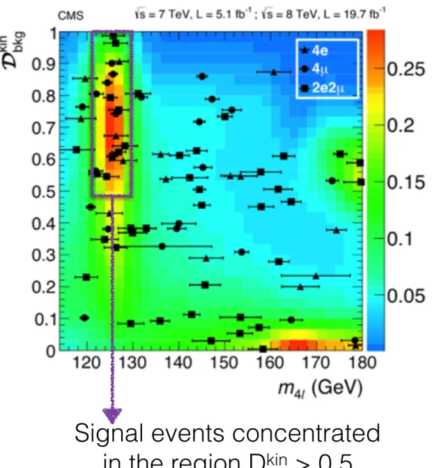
D

v/s m(4ℓ𝓁) distribution

Data overlaid on signal+background prediction

Signal events concentrated in the region D kin > 0.5 Such discriminants also used to measure Higgs

properties like spin-parity, Higgs width

Search Strategy (III)

• Probe the different production modes of the Higgs boson

• Categorize events as dijet-tagged and untagged

• Dijet tagged events : A linear discriminant

constructed using Δη(jj) and m(jj) to separate VBF from gluon fusion

• Untagged events : The p T of the four-lepton system used to discriminate between VBF and gluon fusion

• Search performed using a 3D fit with m(4ℓ𝓁), kinematic discriminant, dijet discriminant (or four-lepton p T )

7

Search Results

8

best-fit values is performed. The mass uncertainty obtained in this way is purely statistical. The systematic uncertainties account for an effect on the mass scale of the lepton momentum scale and resolution, shape systematics in the P ð D kin bkg j m 4l Þ probability density functions used as signal and background models, and normalization systematics due to acceptance and efficiency uncertainty. The measured mass is m H ¼ 125.6 $ 0.4 ð stat Þ $ 0.2 ð syst Þ GeV.

Figure 20 (top) also shows likelihood scans separately for the 4e, 2e2μ, and 4μ final states when using the 3D model L m; 3D Γ of Eq. (14). The measurements in the three

final states are statistically compatible. The best-fit values for each subchannel are also shown in Table VII. The dominant contribution to the systematic uncertainty is the limited knowledge of the lepton momentum scale.

Two more mass measurements are performed with a reduced level of information, by dropping the P ð D kin bkg j m 4l Þ term of the likelihood in Eq. (14), resulting in a 2D model, L m; 2D Γ ≡ L m; 2D Γ ð m 4l ; D m Þ , or by performing only a mass line shape fit and assuming the average mass resolution is applicable for each channel, resulting in a 1D model, L m; 1D Γ ≡ L m; 1D Γ ð m 4l Þ . The measured central value is the same in all three cases, with an increasing uncertainty, due to the reduced information available to the fit in the case of 2D or 1D models. Figure 20 (right) shows the likelihood scans for the combination of all the final states separately for the L m; 1D Γ , L m; 2D Γ , and L m; 3D Γ models.

The mass distribution for the Z → 4l decay exhibits a pronounced resonant peak at m 4l ¼ m Z close to the new boson (80 < m 4l < 100 GeV). Hence, the Z → 4l peak can be used as validation of the measurement of the mass of the new boson using the same techniques as for the Higgs boson. The mass of the reconstructed Z boson in Z → 4l decays, with the assumption of the Particle Data Group (PDG) [149] value for the Z-boson natural width, is consistent in each subchannel. The measured value for the combination of all the Z → 4l final states is m Z ¼ 91.1 GeV, compatible with the PDG value (91.1876 $ 0.0021 GeV) within the total estimated uncertainty of 0.4 GeV [149].

Figure 21 shows the scan of the 3D likelihood versus the width of the SM-like Higgs boson with an arbitrary width.

In this scan, the mass and the signal strength μ are profiled, as all other nuisance parameters. This shows that the data

(GeV) m H

110 120 130 140 150 160 170 180

-value p local

10

10

10

10

10

10

10

10

10 1

= 8 TeV, L = 19.7 fb-1

s

-1 ; = 7 TeV, L = 5.1 fb s

3

5

7

D

Observed

Observed

Observed

Expected

FIG. 19 (color online). Significance of the local excess with respect to the SM background expectation as a function of the Higgs boson mass for the 1D fit (L μ 1D ), the 2D fit (L μ 2D ), and the reference 3D fit (L μ 3D ). Results are shown for the full data sample in the low-mass region only.

(GeV) m H

100 200 300 400 1000

SM σ / σ 95% C.L. limit on

10

1 10

CMS s = 7 TeV, L = 5.1 fb^-1 ; s = 8 TeV, L = 19.7 fb^-1

Observed

Expected without the Higgs boson σ

± 1 Expected

σ

± 2 Expected

(GeV) m H

100 200 300 400 1000

-value p local

10

10

10

10

10

10

10

10

10 1

= 8 TeV, L = 19.7 fb-1

s

-1 ; = 7 TeV, L = 5.1 fb s

D

Observed

Observed

Observed

Expected

3

5

7

FIG. 18 (color online). (top) Observed and expected 95% C.L.

upper limit on the ratio of the production cross section to the SM expectation. The expected 1σ and 2σ ranges of expectation for the background-only model are also shown with green and yellow bands, respectively. (bottom) Significance of the local excess with respect to the SM background expectation as a function of the Higgs boson mass in the full mass range 110 – 1000 GeV.

Results are shown for the 1D fit (L μ 1D ), the 2D fit (L μ 2D ), and the reference 3D fit (L μ 3D ).

S. CHATRCHYAN et al. PHYSICAL REVIEW D 89, 092007 (2014)

092007-26

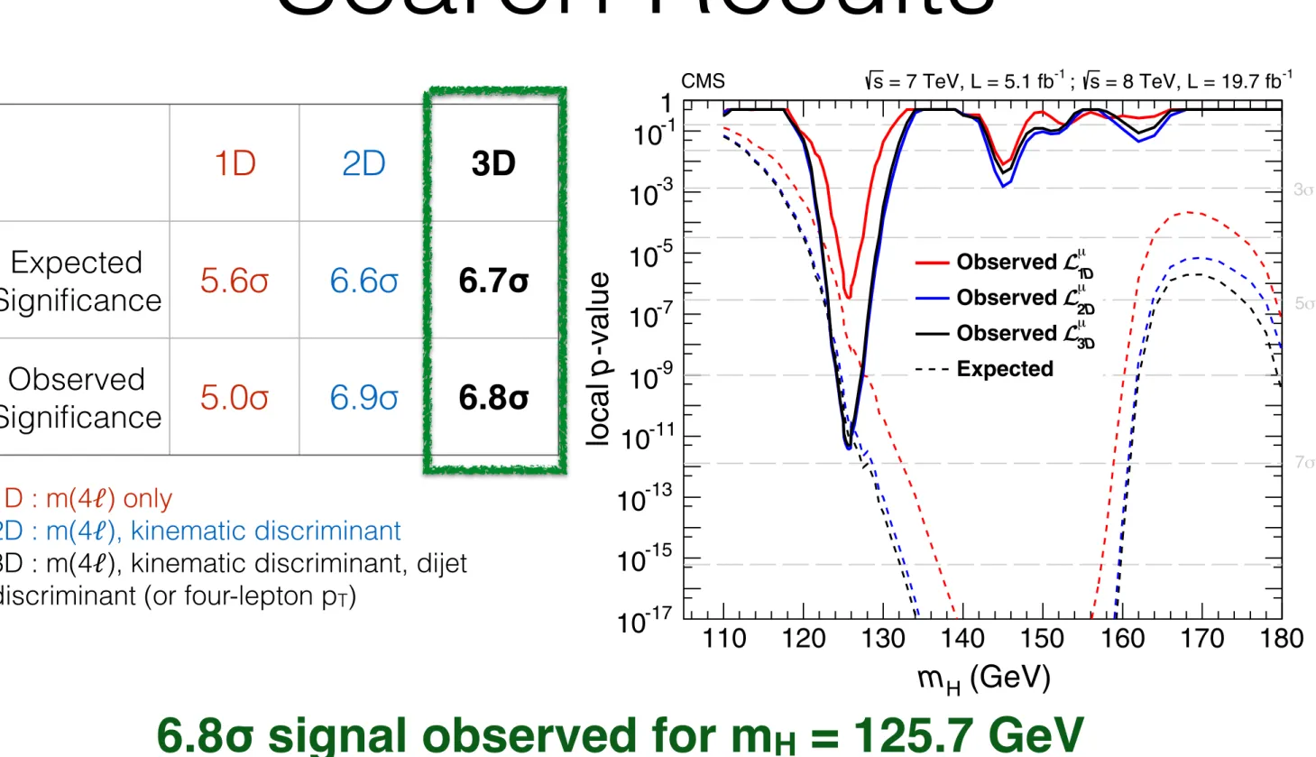
1D 2D 3D

Expected

Significance 5.6σ 6.6σ 6.7σ

Observed

Significance 5.0σ 6.9σ 6.8σ

6.8σ signal observed for m H = 125.7 GeV

Phys. Rev. D 89, 092007 (2014)

1D : m(4ℓ𝓁) only

2D : m(4ℓ𝓁), kinematic discriminant

3D : m(4ℓ𝓁), kinematic discriminant, dijet

discriminant (or four-lepton p

)

Mass Measurement

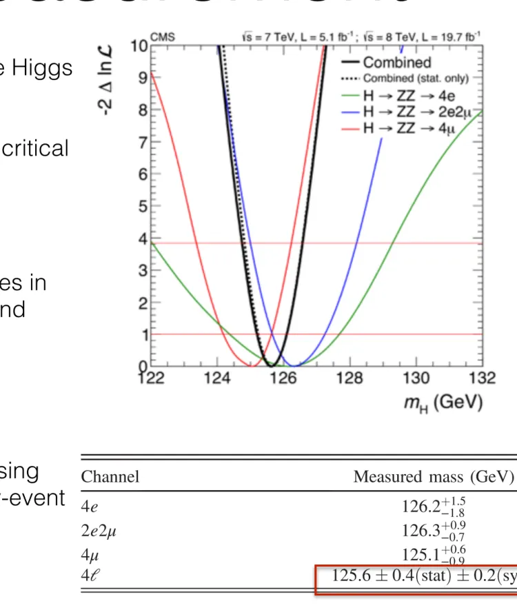
• H→ZZ→4ℓ𝓁 channel is highly sensitive to the Higgs mass

• Precise measurement of lepton momenta is critical

• Multivariate regression used to improve the measurement of electron momentum

• Corrections applied to account for differences in momentum scale/resolution between data and simulation

• Event-by-event mass uncertainties used to optimally exploit the available data

• Mass measurement performed as a 3D fit using m(4ℓ𝓁), kinematic discriminant, and event-by-event mass uncertainties

9

are compatible with a narrow-width resonance. The mea- sured width is Γ

¼ 0.0

GeV, and the upper limit on the width is 3.4 GeV at the 95% C.L. The expected upper limit is 2.8 GeV.

C. Signal strength

The measured signal strength is μ ¼ σ=σ

¼ 0.93

ð stat Þ

ð syst Þ at the best-fit mass (m

¼ 125.6 GeV) with the models of Eqs. (12) and (13) for

the 0/1-jet category and the dijet category, respectively.

The median expected signal strength is μ ¼ 1.00

, for which the total uncertainty agrees with the observed one.

The result is 0.83

in the 0/1-jet category and 1.45

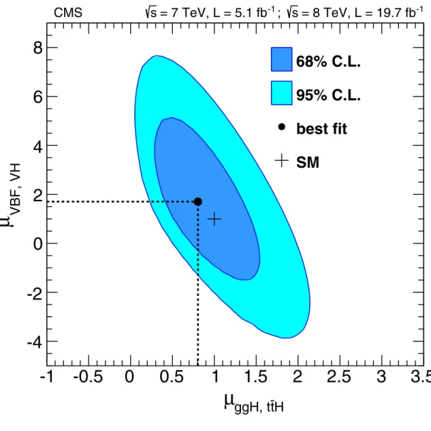
in the dijet category. The best-fit values are shown in Fig. 22 (top). For each category, the signal strength is consistent with SM expectations within the uncertainties, which are dominated by the statistical ones with the current data set.

The categorization according to jet multiplicity and the inclusion of VBF-sensitive variables in the likelihood, like p

and D

, used to measure the cross section in the inclusive category, are also used to disentangle the production mechanisms of the observed new state. The production mechanisms are split into two families depend- ing on whether the production is through couplings to fermions (gluon fusion, t ¯ tH) or vector bosons (VBF, VH).

For m

¼ 126 GeV, about 55% of the VBF events are expected to be included in the dijet category, while only 8%

TABLE VII. Best-fit values for the mass of the Higgs boson candidate, measured in the 4l, l ¼ e; μ final states using a L

model. For the combination of all the final states H → 4l, the separate contributions of the statistical and systematic uncertainty to the total one are given.

Channel Measured mass (GeV)

4e 126.2

2e2μ 126.3

4μ 125.1

4l 125.6 % 0.4 ð stat Þ % 0.2 ð syst Þ

(GeV)

H

0 1 2 3 4 5

ln -2

0 1 2 3 4 5 6

m, D 3

Expected Observed

= 8 TeV, L = 19.7 fb-1

s

-1 ; = 7 TeV, L = 5.1 fb s

CMS

FIG. 21 (color online). Scan of the average expected and observed negative log likelihood − 2 Δ ln L versus the tested SM Higgs boson width Γ

obtained with the 3D fit (L

). The horizontal lines at − 2 Δ ln L ¼ 1 and 3.84 represent the 68% and 95% C.L.’s, respectively.

(GeV) m

ln -2

Combined

Combined (stat. only)

4e ZZ

H ZZ 2e2 H ZZ 4 H

= 8 TeV, L = 19.7 fb-1

s

-1 ; = 7 TeV, L = 5.1 fb s

CMS

(GeV) m

122 124 126 128 130 132

122 124 126 128 130 132

ln -2

(stat. only) = 8 TeV, L = 19.7 fb-1

s

-1 ; = 7 TeV, L = 5.1 fb s

CMS

0 1 2 3 4 5 6 7 8 9 10

0 1 2 3 4 5 6 7 8 9 10

FIG. 20 (color online). (top) Scan of the negative log likelihood

− 2 Δ ln L versus the SM Higgs boson mass m

, for each of the three channels separately and the combination of the three, where the dashed line represents the scan including only statistical uncertainties when using the 3D model. (bottom) Scan of

− 2 Δ ln L versus m

for the combination of the three channels, and using the 1D fit (L

Þ , 2D fit (L

), and 3D fit (L

). The horizontal lines at − 2 Δ ln L ¼ 1 and 3.84 represent the 68% and 95% C.L.’s, respectively.

MEASUREMENT OF THE PROPERTIES OF A HIGGS … PHYSICAL REVIEW D 89, 092007 (2014)

092007-27

Phys. Rev. D 89, 092007 (2014) Dedicated talk on the mass

measurement by M. Sani

Signal Strength

• 3D search analysis allows to disentangle the production modes

• Production modes grouped in two categories:

➡ Vector boson induced (VBF, WH, ZH)

➡ Fermion induced (gluon fusion, ttH)

10

which the total uncertainty agrees with the observed one.

in the 0/1-jet category and 1.45 þ − 0.62 0.89 in the dijet category. The best-fit values are shown in

which the total uncertainty agrees with the observed one.

The result is 0.83 þ − 0.25 0.31

in the dijet category. The best-fit values are shown in

0.93

ð stat Þ

ð syst Þ

125.6 GeV) with the models of Eqs.

VBF,VH ggH,ttH Overall

μ

of the gluon fusion events are included in the dijet category.

As shown in Table V , a fraction of 43% of WH and ZH production contributes to the dijet category. Events that contribute are those in which the vector boson decays hadronically.

Two signal-strength modifiers (μ

and μ

) are introduced as scale factors for the fermion and vector- boson induced contribution to the expected SM cross section. A two-dimensional fit is performed for the two signal-strength modifiers assuming a mass hypothesis of m

¼ 125.6 GeV. The likelihood is profiled for all

nuisance parameters and 68% and 95% C.L. contours in the (μ

; μ

) plane are obtained. Figure 22 (bot- tom) shows the result of the fit leading to the measurements of μ

¼ 0.80

and μ

¼ 1.7

. The mea- sured values are consistent with the expectations for the SM Higgs boson, ð μ

; μ

Þ ¼ ð 1; 1 Þ . With the current limited statistics, we cannot establish yet the presence of VBF and VH production, since μ

¼ 0 is also compatible with the data. Since the decay (into ZZ) is vector-boson mediated, it is necessary that such a coupling must exist in the production side and that the SM VBF and SM VH production mechanisms must be present. The fitted value of μ

larger than 1 is driven partly by the hard p

spectrum of the events observed in data when

µ best fit

0 0.5 1 1.5 2 2.5

0/1-jet Dijet

CMS s = 7 TeV, L = 5.1 fb^-1 ; s = 8 TeV, L = 19.7 fb^-1

H t ggH, t

-1 -0.5 0 0.5 1 µ 1.5 2 2.5 3 3.5

VBF, VH

µ

-4 -2 0 2 4 6

8

95% C.L.

best fit SM

CMS s = 7 TeV, L = 5.1 fb^-1 ; s = 8 TeV, L = 19.7 fb^-1

FIG. 22 (color online). (top) Values of μ for the two categories.

The vertical line shows the combined μ together with its associated

% 1σ uncertainties, shown as a green band. The horizontal bars indicate the % 1σ uncertainties in μ for the different categories. The uncertainties include both statistical and systematic sources of uncertainty. (bottom) Likelihood contours on the signal-strength modifiers associated with fermions (μ

) and vector bosons (μ

) shown at a 68% and 95% C.L.

0 0.1 0.2 0.3 0.4 0.5 0.6 0.7 0.8 0.9 1

Events / 0.05

0 5 10 15 20

25 Data

0

=0

J

* ZZ/Z Z+X

CMS s = 7 TeV, L = 5.1 fb^-1 ; s = 8 TeV, L = 19.7 fb^-1

bkg

0 0.1 0.2 0.3 0.4 0.5 0.6 0.7 0.8 0.9 1

Events / 0.05

0 5 10 15 20

25

(gg)

m (dec)

=2+

JP

* ZZ/Z Z+X

CMS s = 7 TeV, L = 5.1 fb^-1 ; s = 8 TeV, L = 19.7 fb^-1

dec bkg

FIG. 23 (color online). Distribution of D

(top) and D

for the production-independent scenario (bottom) in data and MC expectations for the background and for a signal resonance consistent with the SM Higgs boson with m

¼ 125.6 GeV.

S. CHATRCHYAN et al. PHYSICAL REVIEW D 89, 092007 (2014)

092007-28

Phys. Rev. D 89, 092007 (2014)

Width Measurement

• Measurement of the Higgs width from the observed peak is limited by detector

resolution (~1 GeV)

➡ Width of a 125.6 GeV SM Higgs boson : 4.15 MeV

➡ Direct fit to the signal resonance gives Γ

< 3.4 GeV at 95% CL

• It has been recently shown* that Γ

can be constrained (with mild model dependence) at few 10s of MeV with current data using off-shell signal events

11

Dedicated talk on the width

measurement by L. Quertenmont arxiv:1405.3455 (Accepted by PLB)

*

JHEP 08 116 (2012); Phys. Rev. D 88 054024 (2013);

*

arxiv:1311.3589

Γ H < 33 MeV at 95% CL

1 The discovery of a new boson consistent with the standard model (SM) Higgs boson by the ATLAS and CMS Collaborations was recently reported [1–3]. The mass of the new boson (m

) was measured to be near 125 GeV, and the spin-parity properties were further studied by both experiments, favouring the scalar, J

= 0

, hypothesis [4–7]. The measurement was found to be consistent with a single narrow resonance, and an upper limit of 3.4 GeV at a 95% confidence level (CL) on its decay width (G

) was reported by the CMS experiment in the four-lepton de- cay channel [7]. A direct width measurement at the resonance peak is limited by experimental resolution, and is only sensitive to values far larger than the expected width of around 4 MeV for the SM Higgs boson [8, 9].

It was recently proposed [10] to constrain the Higgs boson width using its off-shell production and decay to two Z bosons away from the resonance peak [11]. In the dominant gluon fusion production mode the off-shell production cross section is known to be sizable. This arises from an enhancement in the decay from the vicinity of the on-shell Z-boson pair production threshold. A further enhancement comes, in gluon fusion production, from the on-shell top- quark pair production threshold. The zero-width approximation is inadequate and the ratio of the off-shell cross section above 2m

to the on-shell signal is of the order of 8% [11, 12]. Further developments to the measurement of the Higgs boson width were proposed in Refs. [13, 14].

The gluon fusion production cross section depends on G

through the Higgs boson propagator ds

dm

⇠ g

2ggH

g

( m

m

)

+ m

G

, (1) where g

and g

are the couplings of the Higgs boson to gluons and Z bosons, respectively.

Integrating in a small region around m

, and above a mass threshold m

> 2m

, where ( m

m

) G

, the cross sections are, respectively,

s

⇠ g

2ggH

g

m

G

and s

⇠ g

2ggH

g

( 2m

)

. (2)

From Eq. (2), it is clear that a measurement of the relative off-shell and on-shell production in the H ! ZZ channel provides direct information on G

, as long as the coupling ratios remain unchanged, i.e. the gluon fusion production is dominated by the top-quark loop and there are no new particles contributing.

The dominant contribution for the production of a pair of Z bosons comes from the quark- initiated process, qq ! ZZ, the diagram for which is displayed in Fig. 1(left). The gluon- induced diboson production involves the gg ! ZZ continuum background production from the box diagrams, as illustrated in Fig. 1(center). An example of the signal production diagram is shown in Fig. 1(right). The interference between the two gluon-induced contributions is significant at high m

[15], and is taken into account in the analysis of the off-shell signal.

Vector boson fusion (VBF) production, which contributes at the level of about 7% to the on- shell cross section, is expected to increase above 2m

. The above formalism describing the ratio of off-shell and on-shell cross sections is applicable to the VBF production mode. In this analysis we constrain the fraction of VBF production using the properties of the events in the on-shell region. The other main Higgs boson production mechanisms, ttH and VH (V=Z,W), which contribute at the level of about 5% to the on-shell signal, are not expected to produce a significant off-shell contribution as they are suppressed at high mass [8, 9]. They are therefore neglected in the off-shell analysis.

In this Letter, we present constraints on the Higgs boson width using its off-shell production

and decay to Z-boson pairs, in the final states where one Z boson decays to an electron or a

Spin-Parity Tests

12

30 6 Results

)

0+ P / L ln(LJ

× -2

-60 -40 -20 0 20 40 60

Pseudoexperiments

0 0.01 0.02 0.03 0.04 0.05 0.06 0.07

CMS(preliminary) 19.7 fb^-1 (8 TeV) + 5.1 fb^-1 (7 TeV)

0+

(dec)

-

2h10

CMS data

P) f(J

0 0.2 0.4 0.6 0.8 1

lnL∆-2

0 5 10 15 20 25 30

→ ZZ

→ X - , gg Expected 2h10

→ ZZ

→ X - , gg Observed 2h10

CMS(preliminary) 19.7 fb^-1 (8 TeV) + 5.1 fb^-1 (7 TeV)

68% CL 95% CL

Figure 12: Distribution of the test statistic q = 2ln(L_J^P/L0⁺) of the hypothesis any ! ²_h10 tested against the SM Higgs boson hypothesis.Distributions for the SM Higgs boson and the alternative J^P hypotheses are represented by the yellow histogram and by the blue histograms, respectively (left). The red arrow indicates the observed value of test-statistics. Expected and observed distribution of 2DlnL for the gg ! ²_h10 model as a function of on the fractional presence f(J^P) of J^P model as a state nearly degenerate with the 0⁺ state (right).

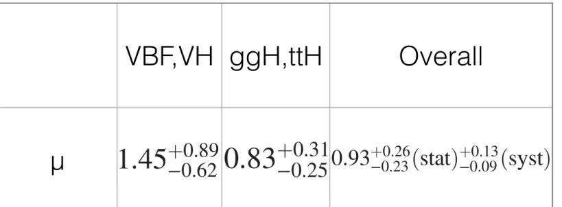
+ h2 2→gg + h3 2→gg + h6 2→gg + h7 2→gg - h9 2→gg - h10 2→gg + h2 2→qq + h3 2→qq + h 2→qq + b 2→qq + h6 2→qq + h7 2→qq - h 2→qq - h9 2→qq - h10 2→qq + h2 2→any + h3 2→any + h 2→any + b 2→any + h6 2→any + h7 2→any - h 2→any - h9 2→any - h10 2→any

)+ 0 /LPJ-2 ln(L

-40 -20 0 20 40 60 80 100

120 CMS(preliminary) 19.7 fb^-1 (8 TeV) + 5.1 fb^-1 (7 TeV)

CMS data Median expected

σ

± 1

0+ J^P± 1σ

σ

± 2

0+ J^P± 2σ

σ

± 3

0+ J^P± 3σ

Figure 13: Summary of the expected and observed values for the test-statistic q distributions for the twelve alternative spin-two hypotheses tested with respect to the SM Higgs boson. The orange (blue) bands represent the 1s, 2s, and 3s around the median expected value for the SM Higgs boson hypothesis (alternative hypothesis). The black point represents the observed value.

CMS-PAS-HIG-14-014

Dedicated talk on spin-parity studies by E. Di Marco

All spin-2 models considered are excluded at 95% CL or higher

• SM Higgs boson expected to be a scalar particle

• This needs to be established in data

• Perform hypothesis tests w.r.t. spin-1 or spin-2 models using dedicated kinematic discriminants

6.2 Constraints on and exclusions of exotic models 29

f

0 0.2 0.4 0.6 0.8 1

)

/ L

ln(L × -2

-20 -10 0 10 20 30 40 50 60

CMS (preliminary) 19.7 fb^-1 (8TeV) + 5.1 fb^-1 (7TeV)

→ x

any

expected σ

± 1

expected σ

± 2 JP

expected σ

± 1

expected σ

± 2 Observed

(a)

f

0 0.2 0.4 0.6 0.8 1

)

/ L

ln(L × -2

-20 -10 0 10 20 30 40 50 60

CMS (preliminary) 19.7 fb^-1 (8TeV) + 5.1 fb^-1 (7TeV)

→ x q

q

expected σ

± 1

expected σ

± 2 JP

expected σ

± 1

expected σ

± 2 Observed

(b)

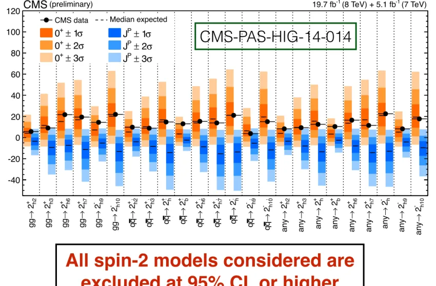
Figure 10: The expected and observed distributions of median test-statistic q for alternative mixed spin-one hypotheses, as a function of f b2 . The green and yellow filled bands represent the 1s and 2s around the median expected value for the SM Higgs boson hypothesis. The red and black dashed bands represent the 1s and 2s around the median expected value for the mixed spin-one hypotheses.

) P f(J

0 0.1 0.2 0.3 0.4 0.5 0.6 0.7 0.8 0.9 1

acceptance) q

(q

-

1

decay-only discriminants

=0.2

f

production q

q

=0.4

f =0.6

f =0.8

f

1

1 =0.2

f =0.4

f =0.6

f =0.8

f

1

σ

± 1 Best-fit

Excluded at 95% CL Expected 95% CL Expected 68% CL

CMS (preliminary) 19.7 fb

(8 TeV) + 5.1 fb

(7 TeV)

Figure 11: Summary expected and observed constraints on the non-interfering fraction mea- surements for the points used in the scan of the f b2 fraction. In the case of production indepen- dent scenarios the f ( J P ) measurement is performed as using the efficiency of qq ! X.

all tested spin-two hypotheses in favour of SM hypothesis 0 + with CL s value larger then 95%

676

CL. The observed non-interfering fraction measurements are summarized in Table 9 and in

677

Figure 14. These results are consistent with the expected SM contribution to the signal. Each

678

of these fractions is tested and reported independently of the other hypotheses, but the reader

679

should note that there are correlations between the various alternate hypotheses.

680

CMS-PAS-HIG-14-014

Any mixture of 1 + and 1 - states excluded at 99% CL or higher

Pure vector Pure

pseudovector

1

/1

Mixture

Probing Spin-0 Couplings

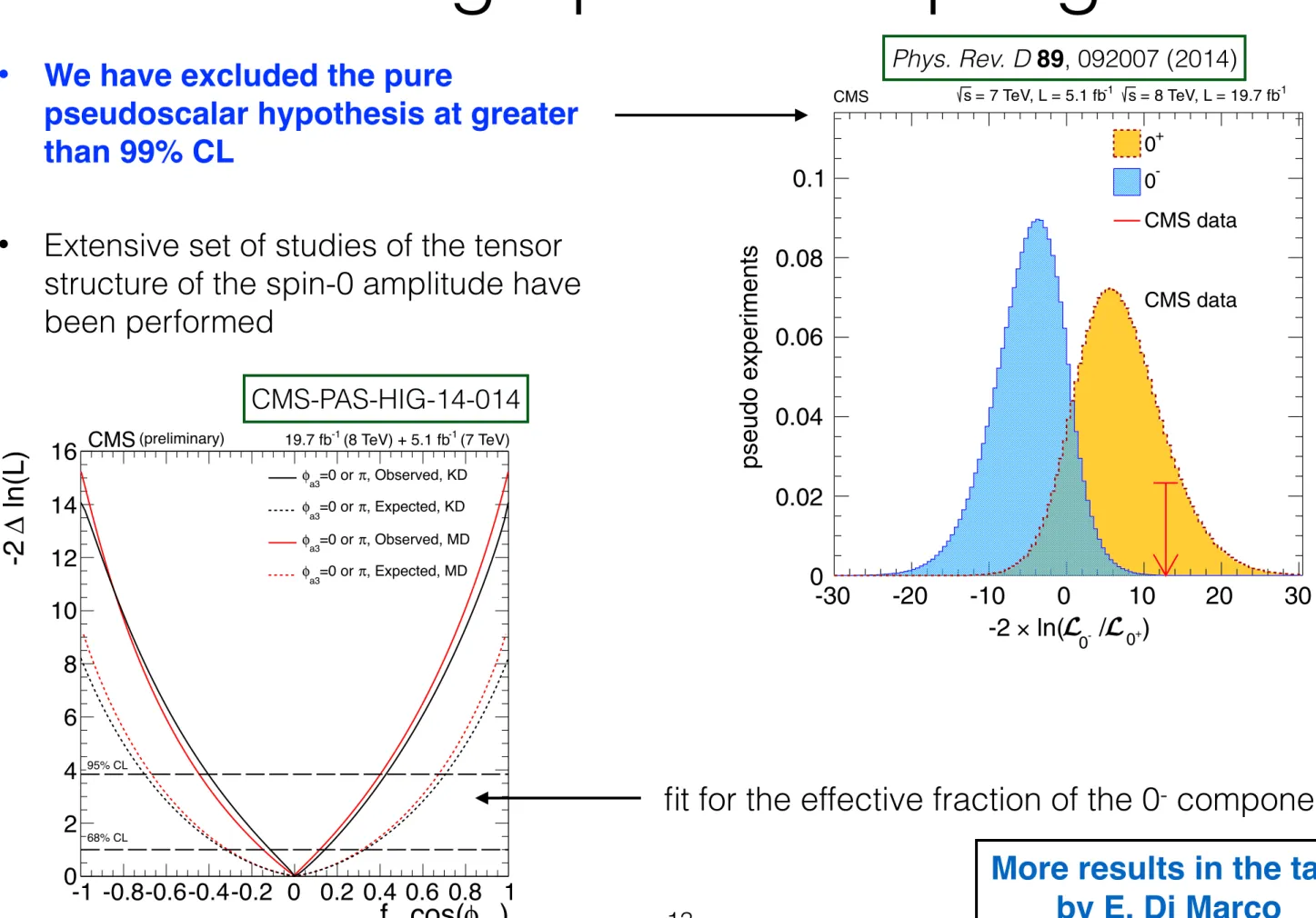
• We have excluded the pure

pseudoscalar hypothesis at greater than 99% CL

• Extensive set of studies of the tensor structure of the spin-0 amplitude have been performed

13

More results in the talk by E. Di Marco

95% or higher C.L. The 0

hypothesis is disfavored, with a CL

value of 4.5%.

In addition to testing pure J

states against the SM Higgs boson hypothesis, a measurement for a possible mixture of CP-even and CP-odd states or other effects leading to anomalous couplings in the H → ZZ decay amplitude in Eq. (6) is performed. The D

discriminant is designed for the discrimination between the third and the first amplitude contributions in Eq. (6) when the phase ϕ

between a

and a

couplings is not determined from the data [48].

For example, even when restricting the coupling ratios to be real, there remains an ambiguity where ϕ

¼ 0 or π.

The interference between the two terms (a

and a

) is found to have a negligible effect on the discriminant distribution or the overall yield of events. The parameter f

is defined as

f

¼ j a

j

σ

j a

j

σ

þ j a

j

σ

þ j a

j

σ

; (18) where σ

is the effective cross section H → ZZ → 2e2μ corresponding to a

¼ 1; a

¼ 0. The 4e and 4μ final

)

0+

/

0-

ln(

-2

-30 -20 -10 0 10 20 30

pseudo experiments

0 0.06 0.08 0.1

CMS s = 7 TeV, L = 5.1 fb^-1 s = 8 TeV, L = 19.7 fb^-1

3

f

0 0.2 0.4 0.6 0.8 1

ln -2

0 2 4 6 8 10 12

Expected Observed

CMS s = 7 TeV, L = 5.1 fb^-1 ; s = 8 TeV, L = 19.7 fb^-1

0+

0-

CMS data

0.04 0.02

CMS data

FIG. 26 (color online). (top) Distribution of the test statistic q ¼ − 2ln ð L

=L

Þ of the pseudoscalar boson hypothesis tested against the SM Higgs boson hypothesis. Distributions for the SM Higgs boson are represented by the yellow histogram, and those for the alternative J

hypotheses are represented by the blue histogram. The arrow indicates the observed value. (bottom) Average expected and observed distribution of − 2 Δ ln L as a function of f

. The horizontal lines at − 2 Δ ln L ¼ 1 and 3.84 represent the 68% and 95% C.L. ’ s, respectively.

TABLE VIII. List of models used in the analysis of the spin and parity hypotheses corresponding to the pure states of the type noted. The expected separation is quoted for two scenarios, where the signal strength for each hypothesis is predetermined from the fit to data and where events are generated with SM expectations for the signal cross section (μ ¼ 1). The observed separation quotes consistency of the observation with the 0

model or J

model and corresponds to the scenario where the signal strength is floated in the fit to data. The last column quotes the CL

value for the J

model.

J

model

J

production

Expected

(μ ¼ 1) Obs. 0

Obs. J

CL

0

any 2.4σ (2.7σ) − 1.0σ þ 3.8σ 0.05%

0

any 1.7σ (1.9σ) − 0.3σ þ 2.1σ 4.5%

1

q q ¯ → X 2.7σ (2.7σ) − 1.4σ þ 4.7σ 0.002%

1

any 2.5σ (2.6σ) − 1.8σ þ 4.9σ 0.001%

1

q q ¯ → X 2.1σ (2.3σ) − 1.5σ þ 4.1σ 0.02%

1

any 2.0σ (2.1σ) − 2.1σ þ 4.8σ 0.004%

2

gg → X 1.9σ (1.8σ) − 1.1σ þ 3.0σ 0.9%

2

q q ¯ → X 1.7σ (1.7σ) − 1.7σ þ 3.8σ 0.2%

2

any 1.5σ (1.5σ) − 1.6σ þ 3.4σ 0.7%

2

gg → X 1.6σ (1.8σ) − 1.4σ þ 3.4σ 0.5%

2

gg → X 3.8σ (4.0σ) þ 1.8σ þ 2.0σ 2.3%

2

gg → X 4.2σ (4.5σ) þ 1.0σ þ 3.2σ 0.09%

-40 -20 0 20 40 60

0-

any

+

0h

any 1-

X q q

1-

any 1+

X q q

1+

any

+m

2 X gg

+m

2 X q q

+m

2 any

+

2b

X gg

+

2h

X gg

-

2h

X gg

CMS s = 7 TeV, L = 5.1 fb^-1; s = 8 TeV, L = 19.7 fb^-1

CMS data Median expected + 1

0 J^P 1

+ 2

0 J^P 2

+ 3

0 J^P 3

FIG. 27 (color online). Summary of the expected and observed values for the test-statistic q distributions for the twelve alter- native hypotheses tested with respect to the SM Higgs boson. The orange (blue) bands represent 1σ, 2σ , and 3σ around the median expected value for the SM Higgs boson hypothesis (alternative hypothesis). The black point represents the observed value.

MEASUREMENT OF THE PROPERTIES OF A HIGGS … PHYSICAL REVIEW D 89, 092007 (2014)

092007-31 Phys. Rev. D 89, 092007 (2014)

19 final state, as it is done for the Z + X background component.

6 Results

In this section we present the results of the study of the Higgs boson interactions with ZZ, Zg ⇤ , and g ⇤ g ⇤ boson pairs, using the analysis approaches described above. In Section 6.1 we study the individual anomalous couplings under the assumption of the spin-zero resonance, as described in Section 2. In case of the HZZ spin-zero interactions we probe both the scenarios where ratios of couplings are considered to be real and the scenarios without this constraint. In case of the spin-zero interactions with Z g ⇤ , and g ⇤ g ⇤ boson pairs, we probe only the scenarios where ratios of couplings are considered to be real. In Section 6.2 we probe several exotic mod- els for the new boson, as discussed in Section 2. The scenarios in which the amplitudes of HZZ spin-zero interactions are considered to be real, we present results from both the kinematic dis- criminant and multidimensional distribution methods. The other studies are performed using the kinematic discriminants method.

In addition, in Section 6.3 we present the results of an extended study of HVV anomalous interactions combining the kinematic discriminant method with results from the H ! WW !

` n ` n decay mode.

6.1 Constraints on spin-zero anomalous couplings

6.1.1 Probing a single spin-zero anomalous coupling

We present the results of the study of HVV interactions under the assumption that the new boson is a spin-zero resonance. Firstly, we consider the constraints that can be put on the presence of only one anomalous term in the HZZ amplitude by maximising the likelihood with respect to the corresponding effective fraction parameter.

a2

) φ

a2

cos(

-1 -0.8-0.6-0.4-0.2 0 0.2 0.4 0.6 0.8 1 f

ln(L) ∆ -2

0 2 4 6 8 10 12 14 16

18

φa2

, Expected, KD π

=0 or φa2

, Observed, MD π

=0 or φa2

, Expected, MD π

=0 or φa2

CMS

68% CL 95% CL

(a)

a3

) φ

a3

cos(

-1 -0.8-0.6-0.4-0.2 0 0.2 0.4 0.6 0.8 1 f

ln(L) ∆ -2

0 2 4 6 8 10 12 14 16

, Observed, KD π

=0 or φa3

, Expected, KD π

=0 or φa3

, Observed, MD π

=0 or φa3

, Expected, MD π

=0 or φa3

CMS

68% CL 95% CL

(b)

Figure 4: Expected and observed likelihood scans for f

(left) and f

(right) obtained using the kinematic discriminant method (KD, black) and multidimensional distribution method (MD, red). The likelihoods are computed assuming the a

/a

and a

/a

coupling ratios are real.

fit for the effective fraction of the 0 - component

CMS-PAS-HIG-14-014

Summary

• A Higgs boson candidate observed in the H→ZZ→4l search with a local significance of 6.8σ

• Several properties of the particle have been measured with this channel

✓ Mass : 125.6±0.4(stat)±0.2(syst) GeV

✓ Signal strength consistent with SM prediction

✓ Width constrained to Γ H < 33 MeV at 95% CL

✓ Spin-parity of the particle consistent with a scalar

• The Higgs boson candidate is consistent with the SM Higgs boson

14

Backup

15

Signal Efficiency

Fraction of signal events selected

Electron Efficiency

Muon Efficiency

16

Kinematic Distributions

Z 1 Mass Z 2 Mass Kinematic

Discriminant

Events in the mass range 121.5-130.5 GeV

17

Four-lepton Mass Distribution

18

Search Results Upto 1 TeV

SM Higgs boson excluded at 95% in the range 114.5-119 GeV and 129.5-832 GeV

Limits p-values

No significant excess except for

m H = 125.7 GeV

Signal Resolution By Channel

20

Mass and On-shell Width Measurement

21

Lepton Scale Uncertainties

Difference in mass scale between data and simulation

Electrons Muons

Estimates of scale uncertainty by channel:

0.1% (4μ), 0.1% (2e2μ), 0.3% (4e)

22

Measurement of Z → 4 ℓ𝓁 Mass Peak

Best fit mass : 91.1 ± 0.4 GeV

23