PDF m.dugi-doc.udg.edu

However, such mechanisms are not effective when large-scale multiple failures arise, that is, when a significant part of the network fails simultaneously. Large-scale failures usually have serious consequences in terms of the economic loss they cause and the disruption they bring to thousands or even millions of users.

Motivation

Almost all recovery techniques focus on individual failures and try to offer some compromise between guarantee of resilience and consumption of resources. It is therefore vital that we have methods and tools that can be applied to the design and operation of communications infrastructure so that essential services can be maintained as much as possible when major failures occur.

Objectives

Outline of the Thesis

• Faults, Errors and Failures
• The concept of Resilience
• Fault Tolerance and Survivability
• Basic Assessment of Resilience

In the network literature, it is common to find terms such as survivability, reliability, fault tolerance, robustness, and dependability. In a recent proposal, it is defined as the ability of a system to fulfill its mission in a timely manner in the presence of threats such as attacks or large-scale natural disasters [129].

Overview of Transport Network Technologies

Wavelength Division Multiplexing

WDM is a technology that allows the transmission of more than one optical signal along a single fiber at the same time. Its principle is essentially the same as frequency division multiplexing (FDM), which means that multiple signals are transmitted using different carriers, each occupying non-overlapping parts of the frequency spectrum [30].

WDM Networks

Light paths can traverse many optical links in a fiber optic network, ideally without OEO conversion. Given that the light path behaves as a pure channel between source and destination, theoretically there is nothing in the signal path to limit the throughput of the fiber [121].

GMPLS-based Networks

Connection-oriented versus Connectionless Networks . 16

The virtual circuit is realized as one or more paths through the network and the data traffic between the two parties flows exclusively through them. "Routers" in a GMPLS-based network forward data based only on labels, so that any layer 3 identifiers (such as IP addresses) that may exist within the protocol's data units are completely ignored.

GMPLS-specific Features

The GMPLS Functional Planes

Network Failure and Recovery

• Types of Physical Failures
• A Failure Taxonomy
• Large-scale Failures
• Categorizing Multiple Failures
• Recovery in GMPLS-based Networks
• Recovery Phases
• Protection and Restoration

It can be argued that such errors are no more than node (hardware) failures due to the fact that the software runs on nodes. In any case, extra traffic may be blocked when failures occur, so it is not protected.

Fundamental Graph Concepts

Graphs and Paths

There can be multiple shortest paths for a given node pair, all of which have the same minimum cost. Two graphsG= (V, E) and G0 = (V0, E0) are isomorphic if they contain the same number of vertices connected in the same way. For example, if the diameter of graphG is four, all graphs that are isomorphic to it have the same diameter.

In research, communication networks are usually modeled as simple, connected, weighted graphs with link capacity and length (eg, distance . in km) as the most common weights.

Basic Graph Features

Metrics and Non-trivial Graph Features

• Degree sequence and Degree distribution
• Path length distribution
• Clustering coefficient
• Measures of Centrality
• Assortativity coefficient
• Algebraic Connectivity and other spectral measurements 43
• Erdős-Rényi Networks
• Generalized Random Networks
• The Watts-Strogatz Small-World Networks
• Scale-free Networks
• Tools and Models for Internet-like Topologies

The path length distribution Pr[HN =k] is the histogram of the length of the shortest path between all possible pairs of nodes in the graph. The study of the path length distribution has helped define the small world network model. In the following subsections, an overview of the models that are more relevant for communication systems is presented.

This results in the introduction of "bridges" that connect initially distant nodes and lead to the shortening of paths in the network.

Measures of Network Robustness

• Network criticality
• Symmetry ratio
• Connectivity and Average two-terminal reliability
• Elasticity
• Viral conductance

However, whether transient disconnection of small network sections is acceptable, as occurs in large data networks such as the Internet, does not provide a meaningful measure. One option is to look at the magnitude of the giant component, but a more flexible alternative is the so-called k-terminal reliability. The use of spectral range as an epidemic threshold is well established in the epidemic literature.

Formally, the viral conductance VC is defined as the area under the curve of the fraction of infected nodes at steady state y∞(s).

Evaluation of topological damage

Size of the largest component

The size of the largest component (alternatively the size of the giant component) is one of the most used measurements, especially in complex networks, see e.g. and the recent study [93]. Fig.4.3 shows the variation observed in the relative size of the largest connected component as more and more links are removed. Initially, when the network is still intact, the size of the largest component corresponds to the network size, i.e. SLC(0) =N.

Therefore, when a number of links are removed, many nodes are very often left isolated in small components (usually of size one or two), reducing the size of the giant component.

Average two-terminal reliability

In general, the difference between the topologies for r <0.15 is small: SLC(rv) is almost linear in all the cases, although with different slopes. An alternative is to replace "remove node x" with "isolate node x" (by removing all its links). We use that approach to explore another aspect not mentioned so far: the variability of the measurements.

On the other hand, cost266x6 is again peculiar in that it is quite stable for r <0.1, but after that point the variation increases rapidly.

Algebraic Connectivity

It is also possible to measure A2T R when removing a node, but this changes N and so the results cannot be related to the original full topology. The less variation the better because it means that no matter which specific elements fail, the performance reduction is expected to be about the same. The bt400 topology is extremely bad, which in this context means that there are some key elements whose failure significantly changes the A2T R.

Evaluation of functional damage

We perform this evaluation on the cost266x6 topology, which performed well in the previous section for small values ​​ofr and is similar in structure to reference transport networks. In order to simulate the provision of service in the network and the occurrence of large-scale failures, an event-driven simulator has been developed that reproduces the process of route selection in a road-oriented transport network. Given the large diameter of the topology, in this experiment we chose to discard traffic that could be considered "local" in the sense of node neighborhood.

It is clear that these figures will be different if the links are equipped with protection, but in any case they emphasize that the functional damage, in this case from the point of view of active links, is much more serious than we can expect if we only look at topological measures alone. such as those evaluated in the previous section.

Limiting functional damage through Link Prioritization

EdgeBC : The betweenness centrality approach

Conversely, a connection is reinserted later when the connections using it are terminated.

OLC : The Observed Link Criticality approach

Performance Comparison

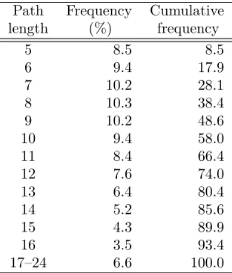
Table 4.2 shows the connection path length frequency distribution of a representative simulation run. Each combination of r, strategy, and z discussed in this section has an entry in the table. Furthermore, due to the nature of the architecture, one failure in the lower layer can manifest as multiple simultaneous failures in higher layers.

In any case, the broader issue of control plane elasticity has not been neglected by the research community, see for example and [79], but is outside the scope of this thesis.

Basic terminology of epidemic networks

A new model of failure propagation: The SID model

SID epidemic thresholds

The spread of the infection in the network depends on the topology of the network via the single parameterλ1 >0. This phenomenon arises from the systematic approach of considering the linearization of the model around the disease-free steady state, where the adjacency matrix of the network appears and the largest eigenvalue λ1 determines the (un)stability. It also analytically shows the values ​​for the number of nodes in the sensitive, infected and disabled states.

The figure highlights two important points: the intersection of the infected and susceptible curves and the intersection of the disabled and susceptible curves.

Empirical validation of the model

1, then the infection dies over time, that is, the number of infected and disabled nodes goes to zero. Finally, for a homogeneous network we have explicit expressions for the endemic steady state: the fraction of susceptible nodes is R1. As time goes by, we can thus have the number of nodes per condition and compare them with the analytical assessment.

As shown in the figure, once the epidemic reaches a steady state, the proportion of infected nodes is close to the analytical value.

Failure propagation on Rings

• Assumptions
• A CTMC model for a small ring
• Guidelines for the assignment of repair rates
• Numerical results

For simplicity, it therefore does not appear in the calculation of the corresponding infection rate. Such a "disconnected" state represents a major malfunction that requires the urgent intervention of the network operator. By solving for the steady state probabilities of the CTMC-based model, it is easy to find the percentage of time the ring remains in each state as a function of the two rectification rates δ1 and δ2.

Severe infection: includes all states where at most one node is disabled and more than half of the nodes are infected.

Comparing robustness against propagating failures

Simulation environment

Thus, the blocking ratio depends only on the effects of the epidemic, which means that connections will only be blocked if there are no viable routes because the necessary intermediate nodes are not available (they are disabled). As for the stages of the SID model, they are chosen so that the topologies to be compared are exposed to infections of similar intensity, which can be easily calculated using the formulations given as part of the SID model definitions.

Measuring the performance degradation

A more stable value is the global or accumulated blocking ratio, identified as “ABP” in Figure 5.10. This happens when the network is in a state where the number of disabled nodes is the maximum possible. Now TRG can be defined in terms of ABP and MBP: TRG is the area between ABP and MBP, once the epidemic reaches its steady state at some point t=k.

However, since MBP and ABP are cumulative values, a simple approximation is the difference between them.

Topology comparison through TRG

The model definition gives us the expression to estimate that number, which means that an additional simulation can be run with that many nodes already disabled. For example, T65 performs better than the others in mild and extreme infections, but is not the best in the rest of the cases. This behavior can be explained by the fact that TRG takes into account not only the speed of the epidemic, but also the connection path lengths.

As can be seen in Appendix B, t65 has a much shorter average path length than the others, and its largest value is between the other two.

Summary

This chapter summarizes the main contributions of this work, along with possible directions for future research. Topology robustness in GMPS networks (TRG) measures how quickly a multiple fault event degrades the performance of the system in terms of its ability to accept connection requests. In the simulation, we carried out a numerical estimation of the number of affected LSPs in a multi-link failure scenario and compared it with the average reliability of two links of the rest of the network to illustrate that topological metrics alone cannot capture the extent of the damage caused at the service level.

Conceptual Framework on Resilience In addition, the thesis presents a comprehensive overview of the terminology on resilience adapted to the needs and applications of the field of networking.

Future work

Betweenness centrality in large complex networks.The European Physical Journal B-Condensed Matter and Complex Systems. In Proceedings of the 1st Annual Workshop on Simplifying Complex Network for Practitioners, SIMPLEX ’09, pages 4:1–4:6. Impact of random failures and attacks on Poisson and power-law random networks.ACM Comput.

Analysis of generalized recovery mechanisms based on GMPLS (including protection and recovery). In Proceedings of the 3rd International Conference on Biology-Inspired Network, Information and Computing Systems Models, BIONETICS ’08, pp. The cost266x6 topology is the result of the juxtaposition of several nearly identical copies of the "Cost266" reference topology, also available on the SNDlib website.

An example of error propagation in a two-component system 7

A schematic representation of an 3x3 optical cross-connect

Example of a logical topology defined over a physical network 15

Example of an MPLS domain

Example of the forwarding table of an MPLS switch

A taxonomy of failures in data networks

The Cost266 topology. Link thickness indicates link importance

An example of random network

An example of Small-World networks

An example of Scale-free networks

Basic operation of DPP. A working path (solid line) and a

Performance comparison of DPP and SPP on four reference

Effect of link failure on the size of the largest component

Effect of node failure on the size of the largest component

Average algebraic connectivity of the largest component

Percentage of connections affected at given fraction of failed

The Control and Data planes in the GMPLS architecture

The state-transition diagram of the SIS model

The eight-node GMPLS-based ring example

Examples of system states on the eight-node ring topology

Robustness comparison of the three studied topologies under

The cost266x6 topology

The bt400 topology

The t204 topology

The er400d3 topology

The er400d6 topology

The eba400h topology

The t65 topology