Persistence in Some Energy Futures Markets

PERSISTENCE IN SOME ENERGY FUTURES MARKETS

JUNCAL CUNADO LUIS A. GIL-ALANA

FERNANDO PÉREZ DE GRACIA

FUNDACIÓN DE LAS CAJAS DE AHORROS DOCUMENTO DE TRABAJO

Nº 434/2008

De conformidad con la base quinta de la convocatoria del Programa de Estímulo a la Investigación, este trabajo ha sido sometido a eva- luación externa anónima de especialistas cualificados a fin de con- trastar su nivel técnico.

ISSN: 1988-8767

La serie DOCUMENTOS DE TRABAJO incluye avances y resultados de investigaciones dentro de los pro- gramas de la Fundación de las Cajas de Ahorros.

Las opiniones son responsabilidad de los autores.

PERSISTENCE IN SOME ENERGY FUTURES MARKETS*

Juncal Cunado Luis A. Gil-Alana Fernando Pérez de Gracia

Abstract

In this paper, we examine the possibility of long range dependence in some energy futures markets for different maturities. In order to test for persistence, we use a variety of techniques based on non-parametric, semiparametric and parametric methods. The results indicate that there is little or no evidence of long memory in gasoline, propane, oil and heating oil at different maturities. However, when we focus on the volatility process, proxied by the absolute returns, we find strong evidence of long memory in all the variables at different contracts.

Key words: Persistence; Long memory; Futures; Energy prices; Volatility.

JEL classification: C32; C59; Q40.

* Juncal Cunado and Luis A. Gil-Alana gratefully acknowledge financial support from the Spanish Ministry of Science and Technology (SEJ2005-07657/ECON). Fernando Pérez de Gracia acknowledges research support from the Spanish Ministry of Science and Technology and FEDER through grant SEJ2005-06302/ECON and from the Plan Especial de Investigación de la Universidad de Navarra.

** Dr. Fernando Pérez de Gracia, Universidad de Navarra -School of Economics and Business -Edificio Biblioteca, Entrada Este -E-31080 Pamplona, SPAIN -Phone: 00 34 948 425 625 -Fax: 00 34 948 425 626 -Email:

[email protected]

1. Introduction

It is commonly accepted that the dynamics of energy prices explain some of the main economic indicators. For example, Hamilton (2008) in a recent survey of the literature on the macroeconomic effects of oil shocks documented that nine out of ten of the US recessions were preceded by increases in the oil price, suggesting then its role as an explanatory variable of economic recessions. Many empirical papers show evidence that energy prices affect macroeconomic variables (e.g., Hamilton, 1983; Hooker, 1996;

Kilian, 2008a,b; Tatom, 1988 and Mork, 1989 among many others). Other studies not only consider the change in oil price as a main determinant of inflation and economic activity but also the oil price volatility as a proxy variable of the level of uncertainty about future oil prices. Papers analysing the relevance of the relationship between oil price volatility and the macroeconomy are Hamilton (1996, 2003) and Guo and Kliesen (2005). Thus, for example, Guo and Kliesen (2005) find that a volatility measure constructed using daily crude oil future prices has a negative and significant effect on GDP growth over the period 1984-2004.

As we have shown in the preceding paragraph, it is relevant to understand the

dynamic behavior of energy prices. In this paper we focus on the persistence in both

energy price returns and their associated volatility processes. Starting with the level of

the series, a number of papers have analyzed mean reversion in energy prices (see, e.g.,

Serletis, 1992; Gil-Alana, 2001 and Postali and Picchetti, 2006). Serletis (1992) using

daily crude oil, heating oil and unleaded gasoline tests for unit roots using standard

methods. His results support the unit root hypothesis when a structural break is taken

into account. More recently, Postali and Piccheti (2006) argue against the existence of

unit roots when a period longer than a century is considered. However, if structural

breaks are taken into account, unit roots remain in shorter periods. Other authors focus the interest on the volatility processes (see, for example, Sadorsky, 2006; Tabak and Cajueiro, 2007 and Elder and Serletis, 2007, 2008 among others). Sadorsky (2006) use univariate and multivariate models to estimate and forecast daily volatility in energy futures prices. Tabak and Cajueiro (2007) also analyze volatility in crude oil markets using long range dependence techniques, based on the rescaled range (R/S) statistic (Hurst, 1951). In another recent paper, Elder and Serletis (2008) test for fractional integration in energy futures markets using semiparametric wavelet estimation methods.

Studies on volatility in futures markets use absolute returns (see, for example, Elder and Jin, 2007) or alternative statistical models (i.e., the family of GARCH models) (see, for example, Sadorsky, 2006).

In a similar vein to the above papers, we also examine the degree of persistence in some energy future markets, using various procedures for estimating and testing long range dependence. We use alternative methods, based on non-parametric (i.e., Lo, 1991, Giraitis et al., 2003), semiparametric (i.e., Robinson, 1995) and parametric (i.e., Sowell, 1992, Robinson, 1994) techniques.

The paper embraces two principal contributions. First, we focus on futures of

energy analyzing persistence in both levels and volatility processes. Previous studies

only focus on prices or volatility. Second, we use three alternative approaches to

document the persistence in futures markets, based on non-parametric, semiparametric

and parametric techniques. It is well known that the results on persistence can

substantially vary depending on the methodology employed. In this respect, the use of a

variety of methods with different distributional assumptions may contribute to

achieving a better overall picture of the degree of persistence of the series.

The structure of the paper is as follows. Section 2 briefly describes the methods of long range dependence that will be employed in the paper. In Section 3, the procedures presented in Section 2 are applied in both the returns and their associated volatility processes. Section 4 contains some concluding comments.

2. Methodology

In this section we present a brief description of the methods employed in Section 3 for estimating and testing long range dependence in some energy futures markets. In all cases we consider the possibility that the underlying model is long memory.

We can provide two definitions of long memory, one in the time domain and the other in the frequency domain. Let us consider a zero-mean process { x

, t

0 ,

1 ,... } with ) γ

E ( x

x

. The time domain definition of long memory states that:

∞

∑^∞ =

−∞

=

u

γ

.

Now, assuming that x

has an absolutely continuous spectral distribution, so that it has spectral density function

, ) ( cos 2 2

) 1 (

0 1 ⎟⎟

⎠

⎜⎜ ⎞

⎝

⎛ + ∑

= ^∞

=

u u u

f

γ γ λ

λ π

the frequency domain definition of long memory states that the spectral density function is unbounded at some frequency in the interval [ 0 ). Most of the empirical work , π carried out so far has concentrated on the case where the singularity or pole in the spectrum takes place at the zero frequency. This is the standard case of

( )

models of the form:

,..., 1 , 0 ,

) 1

(

L

x

u

t

(1)

with d > 0, where L is the lag-operator ( Lx

x

) and u

is

( )

. Note that the polynomial in the left-hand-side in (1) can be expressed in terms of its Binomial expansion, such that, for all real d,

, 2 ...

) 1 1 (

) 1 ( )

1

( ²

0 0

− − +

−

=

∑ ⎟⎟⎠ −

⎜⎜ ⎞

⎝

= ⎛

= ∑

− ^∞

=

∞

= d d L

L d j L

L d

L ^{j j}

j j

j j

d

ψ

and (1) can be written as:

. 2 ....

) 1

(

1

d d x u t

x d

x

If d is an integer value, x

will be a function of a finite number of past observations, while if d is not an integer, x

depends strongly upon values of the time series far away in the past. (See, e.g., Granger and Ding, 1996; Dueker and Startz, 1998). Moreover, the higher the d is, the higher the level of association will be between the observations.

Thus, d is an indicator of the degree of persistence of the series.

The parameter d also plays a crucial role from the statistical viewpoint. Thus, if d = 0, x

is stationary I(0) and is commonly denoted as “short memory”; on the contrary, if d > 0, x

is said to be “long memory” so-named because of the strong degree of association between observations in the far distant past, and if 0 < d < 0.5, the series is still covariance stationary; however, if d ≥ 0.5, the series is no longer stationary and as d increases beyond 0.5 and through 1 the series is becoming “more nonstationary” in the sense, for example, that the partial sums increase in magnitude with d being non- summable. In the following we describe some methods for testing long memory (and fractional integration) in univariate time series.

1 For recent surveys of fractional integration see the papers of Robinson (2003), Doukhan et al. (2003) and more recently, Gil-Alana and Hualde (2008).

2.1 A non-parametric approach

We start with the non-parametric procedures. The two methods presented here test the null hypothesis of short memory (i.e. d = 0 in (1)) against long memory (d > 0) and/or anti-persistence (d < 0). First we describe a procedure developed by Lo (1991). The modified R/S statistic (Lo, 1991) is:

, ) ( min

) ( ) max

ˆ ( ) 1 (

1 1

1 1 ⎟⎟

⎠

⎞

⎜⎜

⎝

⎛ ∑ − − ∑ −

=

≤ =

= ≤

≤

≤

k

j t

T k k

j t

T k T

T

x x x x

q q

Q σ

where

= q

j j j

x

T

q q

1 2

2

( ) ˆ 2 ( ) ˆ ,

ˆ σ ω γ

σ and , 1 ,

1 1 )

( j T

q q j

j ≤ <

− +

ω

and x

is a stationary series (-0.5 < d < 0.5) of sample size T, with sample mean x , sample variance σ ˆ

, and sample autocovariance at lag j given by

This statistic was further normalized as:

T q q Q

V

( )

)

(

. (2)

The null hypothesis of I(0) includes ARMA models, though as pointed out by Haubrich and Lo (2001) does not contain a trend-stationary model. The limiting distribution of V

(q) is derived in Lo (1991) and the 95% confidence interval with equal probabilities in both tails is [0.809, 1.862]. Several Monte Carlo experiments conducted by Teverovsky et al. (1999) and Willinger et al. (1999) show that this method is biased in favor of accepting the null of no long memory as the bandwidth parameter q increases. Therefore, these authors were cautionary about using Lo’s modified method in isolation.

Another recent non-parametric approach is the rescaled-variance V/S statistic

proposed by Giraitis, Kokoszka, Leipus and Teyssiere (2003), which is given by

) , ˆ (

) , ...

, , ) (

(

q T

S S

S q Var

M

T T T

=

σ (3)

where

1

* = ∑ −

= k

j t

k x x

S

and Var ( S

, S

, ... , S

) =

= T

j Sj S

T ₁

*

* )

1 (

is their sample variance. According to Giraitis et al. (2003) the V/S test is more suitable for series that exhibit high volatility, and various Monte Carlo experiments conducted by these authors show that the V/S test is shown to be less sensitive to the choice of the bandwidth number q. The asymptotic distribution of M

(q) coincides with the limiting distribution of the standard Kolmogorov statistic.

A final comment is worthy of mention at this point and it is related with the choice of the optimal bandwidth number q (q

) in the two methods described above: q = 0 correspond to the classic Hurst-Mandelbrot R/S statistic. Haubrich and Lo (2001) suggested using Andrew’s (1991) data-dependent procedure to determine the optimal bandwidth, which is given by

,

2

3

1

* *

⎟⎟

⎠

⎞

⎜⎜

⎝

= ⎛

a T

q (4)

with

,

ˆ ) 1 (

4 ˆ

2 2

* 2

ρ ρ

= −

a

where

is the first order AR coefficient.

2.2 A semi-parametric approach

The method presented here is based on equation (1), where u

is simply supposed to be

I(0). We describe a procedure developed by Robinson (1995), which is essentially a

local ‘Whittle estimator’ in the frequency domain, using a band of frequencies that degenerates to zero. The estimator is implicitly defined by:

, 1 log

2 ) ( log min

ˆ arg

1 ⎟⎟⎠

⎞

⎜⎜⎝

⎛ −

=

∑

= m

s

s

d

C d d m

d λ (5)

, 0 2 ,

, ) 1 (

) (

1

2 = →

= ∑

= T

m T

I s d m

C ^m _s

s

s d s

λ π λ

λ

where I(λ

) is the periodogram of the raw time series, x

, given by:

2 , ) 1 (

2

∑1

= =

T t

st t i

s

x e

I T

λ π

and d ∈ (-0.5, 0.5). Under finiteness of the fourth moment and other mild conditions, Robinson (1995) proved that:

, )

4 / 1 , 0 ( ˆ )

(d − d → N as T → ∞

m _{o d}

where d

is the true value of d.

Though there exist further refinements of this procedure, (Velasco, 1999, Phillips and Shimotsu, 2004, 2005; etc.), these methods require additional user-chosen parameters and then, the results concerning the estimation of d may be very sensitive to the choice of these parameters. In this respect, the method of Robinson (1995) seems computationally simpler.

2.3 A parametric approach

There exist several methods for estimating and testing the fractional differencing parameter in parametric contexts (e.g., Sowell, 1992; Beran, 1993; Tanaka, 1999; etc.).

In this paper we perform a suitable method suggested by Robinson (1994). There are

several reasons for using this method. First, it permits us to include deterministic terms

such as an intercept or a linear time trend unlike what happens with other methods such as Lo’s (1991) non-parametric approach. Another advantage of this method is that it is valid for any real value of d, therefore encompassing stationary (d < 0.5) and nonstationary (d ≥ 0.5) hypotheses, unlike the methods described in Section 2.1 and 2.2 that require first differencing to render the series stationary prior to the estimation of d.

We employ here the following model,

...

, 2 , 1

0 +

,

=

x t

y

β

(6)

,.

..

, 2 , 1 ,

) 1

(

L

x

u

t

(7)

where u

is assumed to be I(0), and given the parametric nature of this method, u

has to have a parametric form, that may be a white noise process, or more generally, allowing some type of weak autocorrelation (i.e, ARMA) structure. In this approach we test the null hypothesis:

,

:

o

d d

H

for any real value d

in (6) and (7), and the limit distribution is standard N(0, 1). The functionial form of the test statistic can be found in any of the numerous empirical applications of his tests (e.g. Gil-Alana and Robinson, 1997, Gil-Alana, 2000, etc.).

3 Evidence of persistence in energy futures markets

The time series data analysed in this section correspond to the log-transformation of daily energy futures prices. All data are obtained from the Energy Information Agency . The sample period for each of the variables is described in Appendix 1.

We use four alternative energy futures prices: crude oil, gasoline, heating oil and

propane. For each variable we have four different maturity contracts. Contract 1 is

defined as a futures contract specifying the earliest delivery date. Contracts 2 to 4

represent the successive delivery months following Contract 1. For detailed information relating to future energy contracts see the Energy Information Agency web site.

Contracts for gasoline, heating oil, and propane expire on the last business day of the month preceding the delivery month. Thus, the delivery month for Contract 1 is the calendar month following the trade date. For crude oil, each contract expires on the third business day prior to the 25

calendar day of the month preceding the delivery month. If the 25

calendar day of the month is a non-business day, trading ceases on the third business day prior to the business day preceding the 25

calendar day. After a contract expires, Contract 1 for the remainder of that calendar month is the second following month.

In this section we examine the possibility of long memory in both the returns and their associated volatility processes in the oil futures with different maturities using alternative methods.

3.1 Persistence in energy future returns

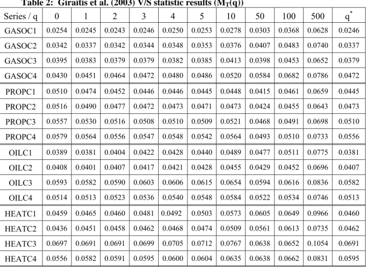
Initially, we implement the test of Lo (1991) described in Section 2.1 to the returns of the four futures of energy prices. Table 1 reports the modified R/S statistic for gasoline, propane, oil and heating oil at different contracts. All futures returns present evidence of I(0) suggesting that the four series are stationary at all contracts. This result holds for all values of the bandwidth number q, including the one based on Andrew’s (1991) procedure in (4). However, using the V/S statistic proposed by Giraitis et al. (2003), (see, Table 2), the results reject the null hypothesis of I(0) processes in all cases.

2 The rejection of the null in the Giraitis et al.’s (2003) procedure may be related with the existence of long memory volatility in the underlying processes. See Section 3.2.

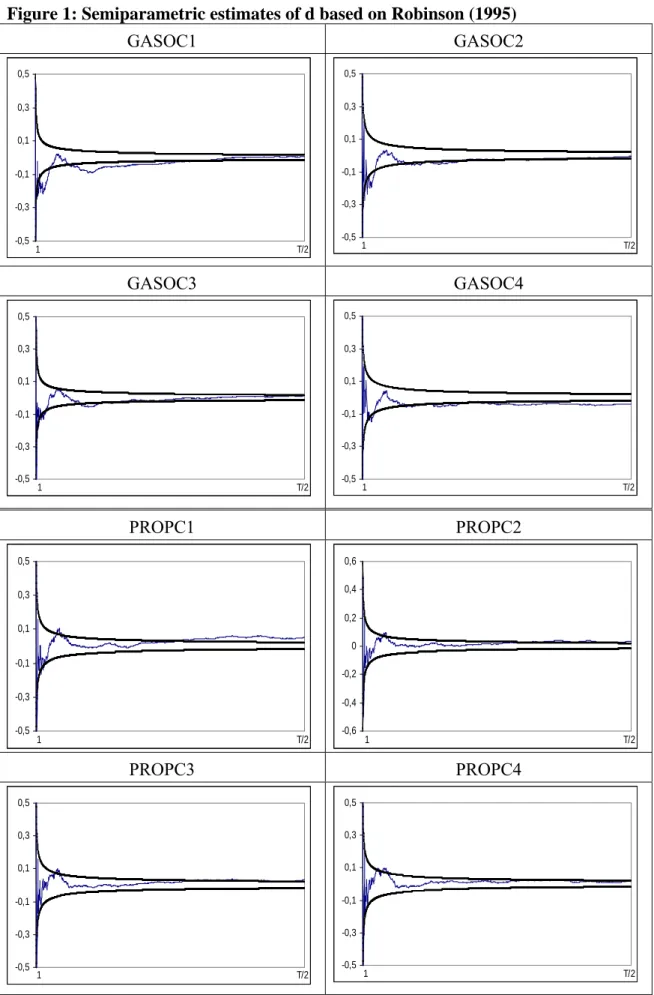
The disparity of the results based on the non-parametric methods suggest that we should try with other approaches. Next we implement the Whittle semiparametric method of Robinson (1995). Figure 1 presents the estimates of d based on Robinson (1995) (see equation (5)) using the whole range of values of the bandwidth number m (displayed in the horizontal axe).

We also display in the plots the 95% confidence interval corresponding to the I(0) case. We find mixed evidence. First, we only find evidence of I(d > 0) for propane in contracts 1 and 2 for some bandwidth numbers.

Second, we obtain some evidence of I(d < 0) (i.e., anti-persistence) in the following cases: contracts 1 and 4 of gasoline, and contract 1 of oil and heating oil. A similar result of anti-persistence is found by Elder and Serletis (2008), showing that the variance of energy futures prices may be dominated by high frequency components.

Finally, for the remaining cases, the estimated values of d are within the I(0) interval.

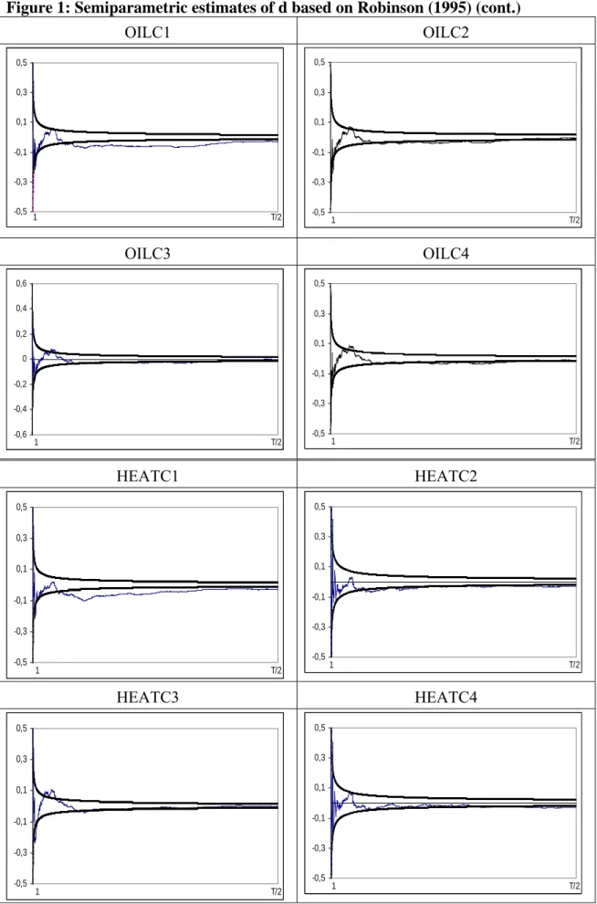
Finally, we use Robinson´s (1994) parametric tests to determine the degree of persistence in the future energy markets. Table 3 reports the results based on white noise, AR(1) and Bloomfield disturbances. The latter is a non-parametric approach of modelling the I(0) disturbances that produce autocorrelations decaying exponentially as in the AR case. Using this method, the first thing we observe is that the results are consistent across the three types of disturbances. We report in the table the estimates of d along with the 95% confidence intervals of the non-rejection values of d.

The I(0) null hypothesis cannot be rejected in many cases and some estimates of d are above 0

3 In case of the Whittle estimator of Robinson (1995), the use of optimal values has not been theoretically justified. Some authors, such as Lobato and Savin (1998) use an interval of values for m. We have preferred to report the results for the whole range of values of m.

4 The confidence intervals were constructed using the following strategy. First, choose a value of d from a grid. Then, form the test statistic testing the null for this value. If the null is rejected at the 95% level, discard this value of d. Otherwise, keep it. An interval is then obtained after considering all the values of d in the grid.

while others are below 0. The main results can be summarized as follows. Firstly, for gasoline, the I(0) hypothesis cannot be rejected in the cases of contracts 1, 2 and 3 if the disturbances are white noise. However, this hypothesis is rejected in favor of a negative d for contract 4 with white noise u

, and for the four gasoline series if the disturbances are autocorrelated. Secondly, for the propane, the estimated d’s are in all cases positive though the I(0) case cannot be rejected in the majority of cases. The exceptions are contracts 1, 2 and 3 with uncorrelated (white noise) errors. Third, for oil prices, we observe negative values of d in practically all cases, and, if u

is autocorrelated the I(0) hypothesis is always rejected in favor of d < 0. Finally, for heating oil, we also obtain negative values of d, but now the I(0) hypothesis is practically never rejected. The exceptions are contract 1 in all cases, and contracts 2 and 4 with white noise u

. Thus, the overall picture in this table indicates that the order of differencing is negative or zero in the majority of the cases.

3.2. Evidence of persistence in volatility

In this sub-section we conduct the same type of analysis as in Section 3.1 but now we focus on the volatility measured as the absolute returns of energy futures prices.

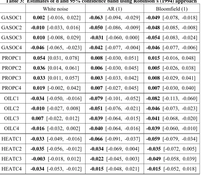
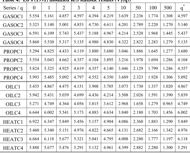
We start again with the non-parametric methods. Using the modified R/S

statistic of Lo (1991) the results for the four series reject the null of I(0) in favour of

long memory behaviour. (see Table 4). Table 5 present the results using the V/S statistic

(Giraitis et al., 2003) and, in this case, the results also support the long memory

hypothesis (I(d, d > 0)) in all series for different maturities.

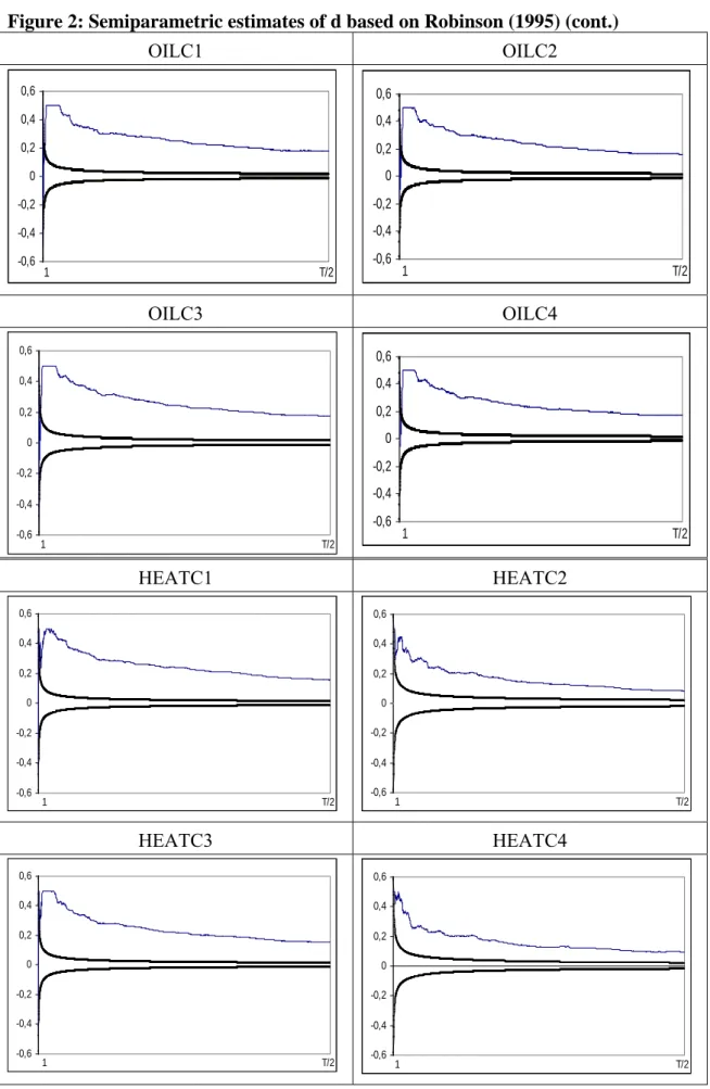
Figure 2 reports the results based on the Whittle semiparametric method of Robinson (1995). We see that for all the variables and contracts, the value of d is found to be statistically significantly above 0, suggesting once more long memory in the volatility process.

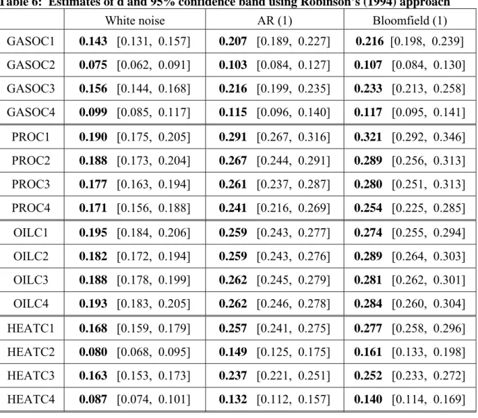
Finally, we perform the parametric procedure of Robinson (1994). For all the energy variables and contracts, the estimates are positive and the intervals exclude the I(0) hypothesis. The lowest degree of persistence in the volatility processes seems to take place for gasoline (contracts 2 and 4) and heating oil (contracts 2 and 4) especially if the disturbances are uncorrelated. On the other extreme, the highest values occur in propane and oil for all different contracts, with values above 0.250 if the disturbances are autocorrelated. The same happens for heating and oil in contract 1.

When we observe the impact of maturity, the results are not very conclusive.

Comparing contracts 1 and 4 across series and types of disturbances, in Table 6, it is observed that the estimated orders of integration in contract 1 are higher than in contract 4 in ten out of the twelve cases presented, however, the overlapping confidence intervals indicate that the results are inconclusive.

4. Conclusions and comments

The dynamic behavior in energy prices is one of the most relevant issues in the global economy. In this paper we have documented evidence of the persistence on futures price returns and volatility in several energy markets (crude oil, gasoline, heating oil and propane) for different maturities. To test this hypothesis we used various alternative

5 Previous studies on volatility in futures markets also use absolute returns (see, for example, Elder and Jin, 2007).

long-range dependence procedures based on non-parametric, semiparametric and parametric techniques.

The main findings of the paper can be summarized as follows: We found little or no evidence of long memory in the energy future prices returns, and this was observed across different maturity rates. However, we found strong evidence of long memory in the volatility processes (measured as absolute returns) in all the four variables. These results are consistent with other financial variables where long range dependence is found exclusively on the volatility processes. When we examine persistence in levels, the estimated values of d are positive for propane and negative for the rest of the variables. We found the highest values of d in contract 1 for propane and oil. If we focus on the volatility processes, the estimated values of d are in all cases positive, and higher for contract 1 in propane and heating oil. In addition, for propane, the persistence decays as the maturity of the contract increases. Finally, the degree of persistence seems to be higher in contract 1 for gasoline, propane and heating oil compared with contract 4.

Long memory is a relevant feature for energy future markets because its

presence can be interpreted as evidence of predictable behavior. Energy price and

volatility persistence are key variables for risk and portfolio managers. Some degree of

predictability would be interpreted as there existing a possibility of exploiting the

dependence in order to generate some extraordinary profits. In this context we find

evidence of some degree of volatility persistence in all energy futures markets. For

example, it seems to be the case that the degree of volatility persistence is higher in the

oil market than in the gasoline market. This result would suggest that there exists more

profit opportunities for investors in oil than in gasoline markets, because there is more

time to respond to changes in volatility in oil than in gasoline.

This paper can be extended in several directions. Thus, longer periods of time can be examined and the possibility of structural breaks should be incorporated into the models. Asymmetric behaviour in energy futures prices is another interesting issue, and models combining fractional integration with non-linearities should be elaborated.

Finally, multivariate models including all future contracts in a single framework will

also be examined in future papers.

References

Andrews, D.W.K., 1991. Heteroskedasticity and autocorrelation consistent covariance matrix estimation. Econometrica 59, 817-858.

Beran, J., 1993, Fitting long memory models by generalized linear regression.

Biometrika 80, 817-822.

Doukhan, P., G. Oppenheim and M.S. Taqqu, 2003. Theory and applications of long range dependence, Birkhäuser, Basel.

Dueker, M. and R. Startz, 1998. Maximum likelihood estimation of fractional cointegration with an application to US and Canadian bond rates. The Review of Economics and Statistics 80, 420-426.

Elder, J. and Jin, H.J., 2007. Long memory in commodity futures volatility: A wavelet perspective. Journal of Futures Markets 27, 411-437.

Elder, J. and Serletis, A., 2008. Long memory in energy futures prices. Review of Financial Economics 17, 146-155.

Energy Information Agency, (

)

Gil-Alana, L.A., 2000. Fractional integration in the purchasing power parity. Economics Letters 69, 285-288.

Gil-Alana, L.A., 2001. A fractionally integrated model with a mean shift for the US and the UK real oil prices. Economic Modelling 18, 643-658.

Gil-Alana, L.A. and J. Hualde, 2008. Fractional integration and cointegration. An overview with an empirical application. The Palgrave Handbook of Applied Econometrics, Volume 2, forthcoming.

Gil-Alana, L.A. and P.M. Robinson, 1997. Testing of unit roots and other nonstationary

hypotheses in macroeconomic time series. Journal of Econometrics 80, 241-268.

Giraitis, L., P. Kokoszka, R. Leipus and G. Teyssiere, 2003. Rescaled variance and related tests for long memory in volatiluty and levels. Journal of Econometrics 112, 265-294.

Granger, C.W.J. and Z. Ding, 1996. Varieties of long memory models. Journal of Econometrics 73, 61-78.

Guo, H. and Kliesen, K.L., 2005. Oil price volatility and US macroeconomic activity.

Federal Reserve Bank of St. Louis Review 11, 669-684.

Hamilton, J., 1983. Oil and the macroeconomy since World War II. Journal of Political Economy 91, 593-617.

Hamilton, J., 1996. This is what happened to the oil price-macroeconomy relationship.

Journal of Monetary Economy 38, 215-220.

Hamilton, J., 2003. What is an oil shock?. Journal of Econometrics 113, 363-398.

Hamilton, J., 2008. Oil and the macroeconomy. New Palgrave Dictionary of Economics, edited by Stephen Durlauf and Lawrence Blume. Forthcoming.

Haubrich, J.G. and Lo, A.W., 2001. The sources and nature of long term memory in aggregate output. Economic Review of the Federal Reserve Bank of Cleveland 37, 15- 30.

Hooker, M., 1996. What happened to the oil price-macroeconomy relationship?.

Journal of Monetary Economics 38, 195-213.

Hurst, H.E., 1951. Long-term storage capacity of reservoirs. Transactions of the American Society Civil Engineers 116, 770-779.

Kilian, L., 2008a. A comparison of the effects of exogenous oil supply shocks on output

and inflation in the G7 countries. Journal of the European Economic Association 6, 78-

121.

Kilian, L., 2008b. Exogenous oil supply shocks: How big are they and how much do they matter for the U.S. economy?. Review of Economics and Statistics 90, 216-240.

Lo, A.W., 1991. Long term memory in stock market prices. Econometrica 59, 1279- 1313,

Lobato, I.N. and N.E. Savin, 1998. Real and spurious long memory properties of stock market data. Journal of Business and Economic Statistics 16, 261-283.

Mork, K., 1989. Oil and the macroeconomy when prices go up and down: An extension of Hamilton´s resuls. Journal of Political Economy 97, 740-744.

Phillips, P.C.B. and K. Shimotsu, 2004. Local Whittle estimation in nonstationary and unit root cases. Annals of Statistics 32, 656-692.

Phillips, P.C.B. and K. Shimotsu, 2005. Exact local Whittle estimation of fractional integration. Annals of Statistics 33, 1890-1933.

Postali, F.A. and Picchetti, P., 2006. Geometric brownian motion and structural breaks in oil prices: A quantitative analysis. Energy Economics 28, 506-522.

Robinson, P.M., 1994. Efficient tests of nonstationary hypotheses. Journal of the American Statistical Association 89, 1420-1437.

Robinson, P.M., 1995. Gaussian semiparametric estimation of long range dependence.

Annals of Statistics 23, 1630-1661.

Robinson, P.M., 2003. Long memory time series, Time Series with Long Memory, (P.M.

Robinson, ed.), Oxford University Press, Oxford, 1-48.

Sadorsky, P., 2006. Modelling and forecasting petroleum futures volatility. Energy Economics 28, 467-488.

Serletis, A., 1992. Unit root behavior in energy futures prices. The Energy Journal 13,

119-128.

Sowell, F., 1992. Maximum likelihood estimation of stationary univariate fractionally integrated time series models. Journal of Econometrics 53, 165-188.

Tabak, B. and Cajueiro, D., 2007. Are the crude oil markets becoming weakly efficient over time? A test for time-varying long-range dependence in prices and volatility.

Energy Economics 29, 28-36.

Tanaka, K., 1999. The nonstationary fractional unit root. Econometric Theory 15, 549- 582.

Tatom, J., 1988. Are the macroeconomic effects of oil price changes symmetric?.

Carnegie - Rochester Conference Series on Public Policy 28, 325-368.

Teverosky, V., M.S. Taqqu and W. Willinger, 1999. A critical look at Lo’s modified R/S statistic. Journal of Statistical Planning and Inference 80, 211-227.

Velasco, C., 1999. Gaussian semiparametric estimation of nonstationary time series, Journal of Time Series Analysis 20, 87-127.

Willinger, W., M.S. Taqqu and V. Teverovsky, 1999. Stock market prices and long

range dependence. Finance and Stochastics 3, 1-13.

Table 1: Lo’s (1991) modified R/S statistic results (V

(q))

Series / q 0 1 2 3 4 5 10 50 100 500 q^*

GASOC1 0.988 0.971 0.967 0.973 0.980 0.987 1.034 1.079 1.190 1.553 0.973 GASOC2 0.945 0.939 0.944 0.947 0.953 0.960 0.991 1.030 1.123 1.390 0.939 GASOC3 1.103 1.086 1.080 1.081 1.085 1.089 1.128 1.106 1.180 1.416 1.081 GASOC4 0.998 1.022 1.037 1.045 1.054 1.061 1.097 1.163 1.257 1.349 1.045 PROPC1 1.323 1.275 1.245 1.237 1.237 1.235 1.240 1.194 1.258 1.503 1.235 PROPC2 1.339 1.305 1.287 1.281 1.282 1.279 1.282 1.214 1.257 1.495 1.282 PROPC3 1.292 1.261 1.245 1.234 1.237 1.235 1.250 1.185 1.213 1.447 1.237 PROPC4 1.241 1.225 1.216 1.206 1.207 1.201 1.224 1.145 1.164 1.396 1.216 OILC1 0.942 0.943 0.961 0.981 0.989 1.001 1.057 1.043 1.081 1.330 0.943 OILC2 1.05 1.043 1.050 1.063 1.068 1.076 1.114 1.078 1.106 1.373 1.050 OILC3 1.127 1.117 1.124 1.136 1.139 1.147 1.183 1.128 1.149 1.338 1.117 OILC4 1.120 1.120 1.130 1.144 1.149 1.157 1.195 1.129 1.142 1.349 1.120 HEATC1 0.981 0.987 0.991 1.004 1.015 1.027 1.096 1.126 1.166 1.423 0.991 HEATC2 1.043 1.061 1.068 1.074 1.081 1.088 1.127 1.183 1.236 1.354 1.074 HEATC3 1.189 1.184 1.184 1.191 1.196 1.206 1.248 1.138 1.150 1.463 1.184 HEATC4 1.127 1.153 1.163 1.166 1.171 1.175 1.205 1.208 1.230 1.378 1.166 The 95% confidence interval for the I(0) null hypothesis is [0.809, 1.862].

Table 2: Giraitis et al. (2003) V/S statistic results (M

(q))

Series / q 0 1 2 3 4 5 10 50 100 500 q

GASOC1 0.0254 0.0245 0.0243 0.0246 0.0250 0.0253 0.0278 0.0303 0.0368 0.0628 0.0246 GASOC2 0.0342 0.0337 0.0342 0.0344 0.0348 0.0353 0.0376 0.0407 0.0483 0.0740 0.0337 GASOC3 0.0395 0.0383 0.0379 0.0379 0.0382 0.0385 0.0413 0.0398 0.0453 0.0652 0.0379 GASOC4 0.0430 0.0451 0.0464 0.0472 0.0480 0.0486 0.0520 0.0584 0.0682 0.0786 0.0472 PROPC1 0.0510 0.0474 0.0452 0.0446 0.0446 0.0445 0.0448 0.0415 0.0461 0.0659 0.0445 PROPC2 0.0516 0.0490 0.0477 0.0472 0.0473 0.0471 0.0473 0.0424 0.0455 0.0643 0.0473 PROPC3 0.0557 0.0530 0.0516 0.0508 0.0510 0.0509 0.0521 0.0468 0.0491 0.0698 0.0510 PROPC4 0.0579 0.0564 0.0556 0.0547 0.0548 0.0542 0.0564 0.0493 0.0510 0.0733 0.0556 OILC1 0.0389 0.0381 0.0404 0.0422 0.0428 0.0440 0.0489 0.0477 0.0511 0.0775 0.0381 OILC2 0.0408 0.0401 0.0407 0.0417 0.0421 0.0428 0.0455 0.0429 0.0452 0.0696 0.0407 OILC3 0.0593 0.0582 0.0590 0.0603 0.0606 0.0615 0.0654 0.0594 0.0616 0.0836 0.0582 OILC4 0.0514 0.0513 0.0523 0.0536 0.0540 0.0548 0.0584 0.0522 0.0534 0.0746 0.0513 HEATC1 0.0459 0.0465 0.0460 0.0481 0.0492 0.0503 0.0573 0.0605 0.0649 0.0966 0.0460 HEATC2 0.0436 0.0451 0.0458 0.0462 0.0468 0.0474 0.0509 0.0561 0.0613 0.0735 0.0462 HEATC3 0.0697 0.0691 0.0691 0.0699 0.0705 0.0712 0.0767 0.0638 0.0652 0.1054 0.0691 HEATC4 0.0556 0.0582 0.0591 0.0595 0.0600 0.0604 0.0635 0.0638 0.0662 0.0831 0.0595 The critical value at the 95% level is 1.36/√T, that is, 0.0183 for GASC1; 0.0239 for GASC2; 0.0183 for ASC3; and 0.0241 for GASC4. 0.0231 for PROC1; 0.0232 for PROC3; and 0.0231 for PROC4. 0.0173 for OILC1; 0.0180 for OILC2; and 0.0180 for OILC4. 0.0163 for HEAC1; 0.0232 for HEAC2; 0.0163 for HEAC3; and 0.0232 for HEAC4.

Figure 1: Semiparametric estimates of d based on Robinson (1995)

GASOC1 GASOC2

-0,5 -0,3 -0,1 0,1 0,3 0,5

1 T/2

-0,5 -0,3 -0,1 0,1 0,3 0,5

1 T/2

GASOC3 GASOC4

-0,5 -0,3 -0,1 0,1 0,3 0,5

1 T/2 ^-0,5

-0,3 -0,1 0,1 0,3 0,5

1 T/2

PROPC1 PROPC2

-0,5 -0,3 -0,1 0,1 0,3 0,5

1 T/2 -0,6

-0,4 -0,2 0 0,2 0,4 0,6

1 T/2

PROPC3 PROPC4

-0,5 -0,3 -0,1 0,1 0,3 0,5

1 T/2

-0,5 -0,3 -0,1 0,1 0,3 0,5

1 T/2

(cont.)

Figure 1: Semiparametric estimates of d based on Robinson (1995) (cont.)

OILC1 OILC2

-0,5 -0,3 -0,1 0,1 0,3 0,5

1 T/2 -0,5

-0,3 -0,1 0,1 0,3 0,5

1 T/2

OILC3 OILC4

-0,6 -0,4 -0,2 0 0,2 0,4 0,6

1 T/2 -0,5

-0,3 -0,1 0,1 0,3 0,5

1 T/2

HEATC1 HEATC2

-0,5 -0,3 -0,1 0,1 0,3 0,5

1 T/2

-0,5 -0,3 -0,1 0,1 0,3 0,5

1 T/2

HEATC3 HEATC4

-0,5 -0,3 -0,1 0,1 0,3 0,5

1 T/2

-0,5 -0,3 -0,1 0,1 0,3 0,5

1 T/2

Table 3: Estimates of d and 95% confidence band using Robinson’s (1994) approach

White noise AR (1) Bloomfield (1)

GASOC1 0.002 [-0.016, 0.022] -0.063 [-0.094, -0.029] -0.049 [-0.078, -0.018]

GASOC2 -0.010 [-0.033, 0.016] -0.050 [-0.086, -0.009] -0.048 [-0.085, -0.008]

GASOC3 0.010 [-0.008, 0.029] -0.031 [-0.060, 0.000] -0.054 [-0.083, -0.024]

GASOC4 -0.046 [-0.065, -0.023] -0.042 [-0.077, -0.004] -0.046 [-0.077, -0.006]

PROPC1 0.054 [0.031, 0.078] 0.008 [-0.030, 0.051] 0.015 [-0.016, 0.048]

PROPC2 0.036 [0.014, 0.061] 0.006 [-0.030, 0.045] 0.005 [-0.026, 0.038]

PROPC3 0.033 [0.011, 0.057] 0.003 [-0.033, 0.042] 0.008 [-0.029, 0.041]

PROPC4 0.019 [-0.002, 0.042] 0.007 [-0.027, 0.045] 0.007 [-0.030, 0.040]

OILC1 -0.034 [-0.050, -0.016] -0.079 [-0.101, -0.052] -0.082 [-0.113, -0.060]

OILC2 -0.010 [-0.027, 0.008] -0.051 [-0.076, -0.021] -0.046 [-0.073, -0.023]

OILC3 0.007 [-0.022, 0.012] -0.039 [-0.064, -0.015] -0.041 [-0.068, -0.020]

OILC4 -0.016 [-0.032, 0.002] -0.040 [-0.064, -0.016] -0.039 [-0.060, -0.010]

HEATC1 -0.033 [-0.049, -0.016] -0.066 [-0.091, -0.037] -0.059 [-0.079, -0.034]

HEATC2 -0.035 [-0.056, -0.012] -0.034 [-0.069, 0.004] -0.035 [-0.072, 0.005]

HEATC3 -0.003 [-0.018, 0.012] -0.022 [-0.045, 0.003] -0.049 [-0.058, 0.039]

HEATC4 -0.034 [-0.053, -0.012] -0.015 [-0.048, 0.021] -0.015 [-0.052, 0.018]

Table 4: Lo’s (1991) modified R/S statistic results (V

(q))

Series / q 0 1 2 3 4 5 10 50 100 500 q

GASOC1

GASOC2

GASOC3

GASOC4

PROPC1

PROPC2

PROPC3

PROPC4

OILC1

OILC2

OILC3

OILC4

HEATC1

HEATC2

HEATC3

HEATC4

Table 5: Giraitis et al. (2003) V/S statistic results (M

(q))

Series / q 0 1 2 3 4 5 10 50 100 500 q

GASOC1

GASOC2

GASOC3

GASOC4

PROPC1

PROPC2

PROPC3

PROPC4

OILC1

OILC2

OILC3

OILC4

HEATC1

HEATC2

HEATC3

HEATC4

Figure 2: Semiparametric estimates of d based on Robinson (1995)

GASOC1 GASOC2

-0,6 -0,4 -0,2 0 0,2 0,4 0,6

1 T/2 -0,6

-0,4 -0,2 0 0,2 0,4 0,6

1 T/2

GASOC3 GASOC4

-0,6 -0,4 -0,2 0 0,2 0,4 0,6

1 T/2

-0,6 -0,4 -0,2 0 0,2 0,4 0,6

1 T/2

PROPC1 PROPC2

-0,6 -0,4 -0,2 0 0,2 0,4 0,6

1 T/2 -0,6

-0,4 -0,2 0 0,2 0,4 0,6

1 T/2

PROPC3 PROPC4

-0,6 -0,4 -0,2 0 0,2 0,4 0,6

1 T/2 -0,6

-0,4 -0,2 0 0,2 0,4 0,6

1 T/2

(cont.)

Figure 2: Semiparametric estimates of d based on Robinson (1995) (cont.)

OILC1 OILC2

-0,6 -0,4 -0,2 0 0,2 0,4 0,6

1 T/2

-0,6 -0,4 -0,2 0 0,2 0,4 0,6

1 T/2

OILC3 OILC4

-0,6 -0,4 -0,2 0 0,2 0,4 0,6

1 T/2

-0,6 -0,4 -0,2 0 0,2 0,4 0,6

1 T/2

HEATC1 HEATC2

-0,6 -0,4 -0,2 0 0,2 0,4 0,6

1 T/2 -0,6

-0,4 -0,2 0 0,2 0,4 0,6

1 T/2

HEATC3 HEATC4

-0,6 -0,4 -0,2 0 0,2 0,4 0,6

1 T/2 -0,6

-0,4 -0,2 0 0,2 0,4 0,6

1 T/2

Table 6: Estimates of d and 95% confidence band using Robinson’s (1994) approach

White noise AR (1) Bloomfield (1)

GASOC1 0.143 [0.131, 0.157] 0.207 [0.189, 0.227] 0.216 [0.198, 0.239]

GASOC2 0.075 [0.062, 0.091] 0.103 [0.084, 0.127] 0.107 [0.084, 0.130]

GASOC3 0.156 [0.144, 0.168] 0.216 [0.199, 0.235] 0.233 [0.213, 0.258]

GASOC4 0.099 [0.085, 0.117] 0.115 [0.096, 0.140] 0.117 [0.095, 0.141]

PROC1 0.190 [0.175, 0.205] 0.291 [0.267, 0.316] 0.321 [0.292, 0.346]

PROC2 0.188 [0.173, 0.204] 0.267 [0.244, 0.291] 0.289 [0.256, 0.313]

PROC3 0.177 [0.163, 0.194] 0.261 [0.237, 0.287] 0.280 [0.251, 0.313]

PROC4 0.171 [0.156, 0.188] 0.241 [0.216, 0.269] 0.254 [0.225, 0.285]

OILC1 0.195 [0.184, 0.206] 0.259 [0.243, 0.277] 0.274 [0.255, 0.294]

OILC2 0.182 [0.172, 0.194] 0.259 [0.243, 0.276] 0.289 [0.264, 0.303]

OILC3 0.188 [0.178, 0.199] 0.262 [0.245, 0.279] 0.281 [0.262, 0.301]

OILC4 0.193 [0.183, 0.205] 0.262 [0.246, 0.278] 0.284 [0.260, 0.304]

HEATC1 0.168 [0.159, 0.179] 0.257 [0.241, 0.275] 0.277 [0.258, 0.296]

HEATC2 0.080 [0.068, 0.095] 0.149 [0.125, 0.175] 0.161 [0.133, 0.198]

HEATC3 0.163 [0.153, 0.173] 0.237 [0.221, 0.251] 0.252 [0.233, 0.272]

HEATC4 0.087 [0.074, 0.101] 0.132 [0.112, 0.157] 0.140 [0.114, 0.169]

Appendix 1.

Sample period

Starting date Ending date Number of Observations Gasoline

Contract 1 January 02, 1985 December 29, 2006 5514 Contract 2 January 20, 1994 November 30, 2006 3218 Contract 3 December 03, 1984 October 31, 2006 5492 Contract 4 January 28, 1994 September 29, 2006 3170

Propane

Contract 1 December 17, 1993 October 02, 2007 3447 Contract 2 February 02, 1994 October 02, 2007 3416 Contract 3 February 08, 1994 October 02, 2007 3412 Contract 4 December 17, 1993 October 02, 2007 3447

Oil

Contract 1 April 04, 1983 October 02, 1985 6143 Contract 2 January 02, 1985 October 02, 2007 5705 Contract 3 March 30, 1983 October 02, 2007 6145 Contract 4 January 02, 1985 October 02, 2007 5705

Heating Oil

Contract 1 January 02, 1980 October 02, 2007 6159 Contract 2 February 02, 1994 October 02, 2007 3418 Contract 3 January 02, 1980 October 02, 2007 6159 Contract 4 January 14, 1994 October 02, 2007 3433

F

C

A

Últimos números publicados

159/2000 Participación privada en la construcción y explotación de carreteras de peaje Ginés de Rus, Manuel Romero y Lourdes Trujillo

160/2000 Errores y posibles soluciones en la aplicación del Value at Risk Mariano González Sánchez

161/2000 Tax neutrality on saving assets. The spahish case before and after the tax reform Cristina Ruza y de Paz-Curbera

162/2000 Private rates of return to human capital in Spain: new evidence F. Barceinas, J. Oliver-Alonso, J.L. Raymond y J.L. Roig-Sabaté 163/2000 El control interno del riesgo. Una propuesta de sistema de límites

riesgo neutral

Mariano González Sánchez

164/2001 La evolución de las políticas de gasto de las Administraciones Públicas en los años 90 Alfonso Utrilla de la Hoz y Carmen Pérez Esparrells

165/2001 Bank cost efficiency and output specification Emili Tortosa-Ausina

166/2001 Recent trends in Spanish income distribution: A robust picture of falling income inequality Josep Oliver-Alonso, Xavier Ramos y José Luis Raymond-Bara

167/2001 Efectos redistributivos y sobre el bienestar social del tratamiento de las cargas familiares en el nuevo IRPF

Nuria Badenes Plá, Julio López Laborda, Jorge Onrubia Fernández

168/2001 The Effects of Bank Debt on Financial Structure of Small and Medium Firms in some Euro- pean Countries

Mónica Melle-Hernández

169/2001 La política de cohesión de la UE ampliada: la perspectiva de España Ismael Sanz Labrador

170/2002 Riesgo de liquidez de Mercado Mariano González Sánchez

171/2002 Los costes de administración para el afiliado en los sistemas de pensiones basados en cuentas de capitalización individual: medida y comparación internacional.

José Enrique Devesa Carpio, Rosa Rodríguez Barrera, Carlos Vidal Meliá

172/2002 La encuesta continua de presupuestos familiares (1985-1996): descripción, representatividad y propuestas de metodología para la explotación de la información de los ingresos y el gasto.

Llorenc Pou, Joaquín Alegre

173/2002 Modelos paramétricos y no paramétricos en problemas de concesión de tarjetas de credito.

Rosa Puertas, María Bonilla, Ignacio Olmeda

174/2002 Mercado único, comercio intra-industrial y costes de ajuste en las manufacturas españolas.

José Vicente Blanes Cristóbal

175/2003 La Administración tributaria en España. Un análisis de la gestión a través de los ingresos y de los gastos.

Juan de Dios Jiménez Aguilera, Pedro Enrique Barrilao González 176/2003 The Falling Share of Cash Payments in Spain.

Santiago Carbó Valverde, Rafael López del Paso, David B. Humphrey Publicado en “Moneda y Crédito” nº 217, pags. 167-189.

177/2003 Effects of ATMs and Electronic Payments on Banking Costs: The Spanish Case.

Santiago Carbó Valverde, Rafael López del Paso, David B. Humphrey

178/2003 Factors explaining the interest margin in the banking sectors of the European Union.

Joaquín Maudos y Juan Fernández Guevara

179/2003 Los planes de stock options para directivos y consejeros y su valoración por el mercado de valores en España.

Mónica Melle Hernández

180/2003 Ownership and Performance in Europe and US Banking – A comparison of Commercial, Co- operative & Savings Banks.

Yener Altunbas, Santiago Carbó y Phil Molyneux

181/2003 The Euro effect on the integration of the European stock markets.

Mónica Melle Hernández

182/2004 In search of complementarity in the innovation strategy: international R&D and external knowledge acquisition.

Bruno Cassiman, Reinhilde Veugelers

183/2004 Fijación de precios en el sector público: una aplicación para el servicio municipal de sumi- nistro de agua.

Mª Ángeles García Valiñas

184/2004 Estimación de la economía sumergida es España: un modelo estructural de variables latentes.

Ángel Alañón Pardo, Miguel Gómez de Antonio

185/2004 Causas políticas y consecuencias sociales de la corrupción.

Joan Oriol Prats Cabrera

186/2004 Loan bankers’ decisions and sensitivity to the audit report using the belief revision model.

Andrés Guiral Contreras and José A. Gonzalo Angulo

187/2004 El modelo de Black, Derman y Toy en la práctica. Aplicación al mercado español.

Marta Tolentino García-Abadillo y Antonio Díaz Pérez 188/2004 Does market competition make banks perform well?.

Mónica Melle

189/2004 Efficiency differences among banks: external, technical, internal, and managerial Santiago Carbó Valverde, David B. Humphrey y Rafael López del Paso

190/2004 Una aproximación al análisis de los costes de la esquizofrenia en españa: los modelos jerár- quicos bayesianos

F. J. Vázquez-Polo, M. A. Negrín, J. M. Cavasés, E. Sánchez y grupo RIRAG 191/2004 Environmental proactivity and business performance: an empirical analysis

Javier González-Benito y Óscar González-Benito

192/2004 Economic risk to beneficiaries in notional defined contribution accounts (NDCs) Carlos Vidal-Meliá, Inmaculada Domínguez-Fabian y José Enrique Devesa-Carpio

193/2004 Sources of efficiency gains in port reform: non parametric malmquist decomposition tfp in- dex for Mexico

Antonio Estache, Beatriz Tovar de la Fé y Lourdes Trujillo 194/2004 Persistencia de resultados en los fondos de inversión españoles

Alfredo Ciriaco Fernández y Rafael Santamaría Aquilué

195/2005 El modelo de revisión de creencias como aproximación psicológica a la formación del juicio del auditor sobre la gestión continuada

Andrés Guiral Contreras y Francisco Esteso Sánchez

196/2005 La nueva financiación sanitaria en España: descentralización y prospectiva David Cantarero Prieto

197/2005 A cointegration analysis of the Long-Run supply response of Spanish agriculture to the com- mon agricultural policy

José A. Mendez, Ricardo Mora y Carlos San Juan

198/2005 ¿Refleja la estructura temporal de los tipos de interés del mercado español preferencia por la li- quidez?

Magdalena Massot Perelló y Juan M. Nave

199/2005 Análisis de impacto de los Fondos Estructurales Europeos recibidos por una economía regional:

Un enfoque a través de Matrices de Contabilidad Social M. Carmen Lima y M. Alejandro Cardenete

200/2005 Does the development of non-cash payments affect monetary policy transmission?

Santiago Carbó Valverde y Rafael López del Paso

201/2005 Firm and time varying technical and allocative efficiency: an application for port cargo han- dling firms

Ana Rodríguez-Álvarez, Beatriz Tovar de la Fe y Lourdes Trujillo 202/2005 Contractual complexity in strategic alliances

Jeffrey J. Reuer y Africa Ariño

203/2005 Factores determinantes de la evolución del empleo en las empresas adquiridas por opa Nuria Alcalde Fradejas y Inés Pérez-Soba Aguilar

204/2005 Nonlinear Forecasting in Economics: a comparison between Comprehension Approach versus Learning Approach. An Application to Spanish Time Series

Elena Olmedo, Juan M. Valderas, Ricardo Gimeno and Lorenzo Escot

205/2005 Precio de la tierra con presión urbana: un modelo para España Esther Decimavilla, Carlos San Juan y Stefan Sperlich

206/2005 Interregional migration in Spain: a semiparametric analysis Adolfo Maza y José Villaverde

207/2005 Productivity growth in European banking

Carmen Murillo-Melchor, José Manuel Pastor y Emili Tortosa-Ausina

208/2005 Explaining Bank Cost Efficiency in Europe: Environmental and Productivity Influences.

Santiago Carbó Valverde, David B. Humphrey y Rafael López del Paso

209/2005 La elasticidad de sustitución intertemporal con preferencias no separables intratemporalmente: los casos de Alemania, España y Francia.

Elena Márquez de la Cruz, Ana R. Martínez Cañete y Inés Pérez-Soba Aguilar

210/2005 Contribución de los efectos tamaño, book-to-market y momentum a la valoración de activos: el caso español.

Begoña Font-Belaire y Alfredo Juan Grau-Grau

211/2005 Permanent income, convergence and inequality among countries José M. Pastor and Lorenzo Serrano

212/2005 The Latin Model of Welfare: Do ‘Insertion Contracts’ Reduce Long-Term Dependence?

Luis Ayala and Magdalena Rodríguez

213/2005 The effect of geographic expansion on the productivity of Spanish savings banks Manuel Illueca, José M. Pastor and Emili Tortosa-Ausina

214/2005 Dynamic network interconnection under consumer switching costs Ángel Luis López Rodríguez

215/2005 La influencia del entorno socioeconómico en la realización de estudios universitarios: una aproxi- mación al caso español en la década de los noventa

Marta Rahona López

216/2005 The valuation of spanish ipos: efficiency analysis Susana Álvarez Otero

217/2005 On the generation of a regular multi-input multi-output technology using parametric output dis- tance functions

Sergio Perelman and Daniel Santin

218/2005 La gobernanza de los procesos parlamentarios: la organización industrial del congreso de los di- putados en España

Gonzalo Caballero Miguez

219/2005 Determinants of bank market structure: Efficiency and political economy variables Francisco González

220/2005 Agresividad de las órdenes introducidas en el mercado español: estrategias, determinantes y me- didas de performance

David Abad Díaz

221/2005 Tendencia post-anuncio de resultados contables: evidencia para el mercado español Carlos Forner Rodríguez, Joaquín Marhuenda Fructuoso y Sonia Sanabria García 222/2005 Human capital accumulation and geography: empirical evidence in the European Union

Jesús López-Rodríguez, J. Andrés Faíña y Jose Lopez Rodríguez

223/2005 Auditors' Forecasting in Going Concern Decisions: Framing, Confidence and Information Proc- essing

Waymond Rodgers and Andrés Guiral

224/2005 The effect of Structural Fund spending on the Galician region: an assessment of the 1994-1999 and 2000-2006 Galician CSFs

José Ramón Cancelo de la Torre, J. Andrés Faíña and Jesús López-Rodríguez

225/2005 The effects of ownership structure and board composition on the audit committee activity: Span- ish evidence

Carlos Fernández Méndez and Rubén Arrondo García

226/2005 Cross-country determinants of bank income smoothing by managing loan loss provisions Ana Rosa Fonseca and Francisco González

227/2005 Incumplimiento fiscal en el irpf (1993-2000): un análisis de sus factores determinantes Alejandro Estellér Moré

228/2005 Region versus Industry effects: volatility transmission Pilar Soriano Felipe and Francisco J. Climent Diranzo

229/2005 Concurrent Engineering: The Moderating Effect Of Uncertainty On New Product Development Success

Daniel Vázquez-Bustelo and Sandra Valle

230/2005 On zero lower bound traps: a framework for the analysis of monetary policy in the ‘age’ of cen- tral banks

Alfonso Palacio-Vera

231/2005 Reconciling Sustainability and Discounting in Cost Benefit Analysis: a methodological proposal M. Carmen Almansa Sáez and Javier Calatrava Requena

232/2005 Can The Excess Of Liquidity Affect The Effectiveness Of The European Monetary Policy?

Santiago Carbó Valverde and Rafael López del Paso

233/2005 Inheritance Taxes In The Eu Fiscal Systems: The Present Situation And Future Perspectives.

Miguel Angel Barberán Lahuerta

234/2006 Bank Ownership And Informativeness Of Earnings.

Víctor M. González

235/2006 Developing A Predictive Method: A Comparative Study Of The Partial Least Squares Vs Maxi- mum Likelihood Techniques.

Waymond Rodgers, Paul Pavlou and Andres Guiral.

236/2006 Using Compromise Programming for Macroeconomic Policy Making in a General Equilibrium Framework: Theory and Application to the Spanish Economy.

Francisco J. André, M. Alejandro Cardenete y Carlos Romero.

237/2006 Bank Market Power And Sme Financing Constraints.

Santiago Carbó-Valverde, Francisco Rodríguez-Fernández y Gregory F. Udell.

238/2006 Trade Effects Of Monetary Agreements: Evidence For Oecd Countries.

Salvador Gil-Pareja, Rafael Llorca-Vivero y José Antonio Martínez-Serrano.

239/2006 The Quality Of Institutions: A Genetic Programming Approach.

Marcos Álvarez-Díaz y Gonzalo Caballero Miguez.

240/2006 La interacción entre el éxito competitivo y las condiciones del mercado doméstico como deter- minantes de la decisión de exportación en las Pymes.

Francisco García Pérez.

241/2006 Una estimación de la depreciación del capital humano por sectores, por ocupación y en el tiempo.

Inés P. Murillo.

242/2006 Consumption And Leisure Externalities, Economic Growth And Equilibrium Efficiency.

Manuel A. Gómez.

243/2006 Measuring efficiency in education: an analysis of different approaches for incorporating non-discretionary inputs.

Jose Manuel Cordero-Ferrera, Francisco Pedraja-Chaparro y Javier Salinas-Jiménez

244/2006 Did The European Exchange-Rate Mechanism Contribute To The Integration Of Peripheral Countries?.

Salvador Gil-Pareja, Rafael Llorca-Vivero y José Antonio Martínez-Serrano 245/2006 Intergenerational Health Mobility: An Empirical Approach Based On The Echp.

Marta Pascual and David Cantarero

246/2006 Measurement and analysis of the Spanish Stock Exchange using the Lyapunov exponent with digital technology.

Salvador Rojí Ferrari and Ana Gonzalez Marcos

247/2006 Testing For Structural Breaks In Variance Withadditive Outliers And Measurement Errors.

Paulo M.M. Rodrigues and Antonio Rubia

248/2006 The Cost Of Market Power In Banking: Social Welfare Loss Vs. Cost Inefficiency.

Joaquín Maudos and Juan Fernández de Guevara

249/2006 Elasticidades de largo plazo de la demanda de vivienda: evidencia para España (1885-2000).

Desiderio Romero Jordán, José Félix Sanz Sanz y César Pérez López 250/2006 Regional Income Disparities in Europe: What role for location?.

Jesús López-Rodríguez and J. Andrés Faíña

251/2006 Funciones abreviadas de bienestar social: Una forma sencilla de simultanear la medición de la eficiencia y la equidad de las políticas de gasto público.

Nuria Badenes Plá y Daniel Santín González

252/2006 “The momentum effect in the Spanish stock market: Omitted risk factors or investor behaviour?”.

Luis Muga and Rafael Santamaría

253/2006 Dinámica de precios en el mercado español de gasolina: un equilibrio de colusión tácita.

Jordi Perdiguero García

254/2006 Desigualdad regional en España: renta permanente versus renta corriente.

José M.Pastor, Empar Pons y Lorenzo Serrano

255/2006 Environmental implications of organic food preferences: an application of the impure public goods model.

Ana Maria Aldanondo-Ochoa y Carmen Almansa-Sáez

256/2006 Family tax credits versus family allowances when labour supply matters: Evidence for Spain.

José Felix Sanz-Sanz, Desiderio Romero-Jordán y Santiago Álvarez-García

257/2006 La internacionalización de la empresa manufacturera española: efectos del capital humano genérico y específico.

José López Rodríguez

258/2006 Evaluación de las migraciones interregionales en España, 1996-2004.

María Martínez Torres

259/2006 Efficiency and market power in Spanish banking.

Rolf Färe, Shawna Grosskopf y Emili Tortosa-Ausina.

260/2006 Asimetrías en volatilidad, beta y contagios entre las empresas grandes y pequeñas cotizadas en la bolsa española.

Helena Chuliá y Hipòlit Torró.

261/2006 Birth Replacement Ratios: New Measures of Period Population Replacement.

José Antonio Ortega.

262/2006 Accidentes de tráfico, víctimas mortales y consumo de alcohol.

José Mª Arranz y Ana I. Gil.

263/2006 Análisis de la Presencia de la Mujer en los Consejos de Administración de las Mil Mayores Em- presas Españolas.

Ruth Mateos de Cabo, Lorenzo Escot Mangas y Ricardo Gimeno Nogués.

264/2006 Crisis y Reforma del Pacto de Estabilidad y Crecimiento. Las Limitaciones de la Política Econó- mica en Europa.

Ignacio Álvarez Peralta.

265/2006 Have Child Tax Allowances Affected Family Size? A Microdata Study For Spain (1996-2000).

Jaime Vallés-Giménez y Anabel Zárate-Marco.

266/2006 Health Human Capital And The Shift From Foraging To Farming.

Paolo Rungo.

267/2006 Financiación Autonómica y Política de la Competencia: El Mercado de Gasolina en Canarias.

Juan Luis Jiménez y Jordi Perdiguero.

268/2006 El cumplimiento del Protocolo de Kyoto para los hogares españoles: el papel de la imposición sobre la energía.

Desiderio Romero-Jordán y José Félix Sanz-Sanz.

269/2006 Banking competition, financial dependence and economic growth Joaquín Maudos y Juan Fernández de Guevara

270/2006 Efficiency, subsidies and environmental adaptation of animal farming under CAP Werner Kleinhanß, Carmen Murillo, Carlos San Juan y Stefan Sperlich

271/2006 Interest Groups, Incentives to Cooperation and Decision-Making Process in the European Union A. Garcia-Lorenzo y Jesús López-R