POLICY SUCCESS OR ECONOMIC SLOWDOWN?
EFFECTS OF THE 80 KM•H-1 SPEED LIMIT ON AIR POLLUTION IN THE BARCELONA
METROPOLITAN AREA
GERMÀ BEL I QUERALT JORDI ROSELL I SEGURA
FUNDACIÓN DE LAS CAJAS DE AHORROS DOCUMENTO DE TRABAJO
Nº 663/2011
De conformidad con la base quinta de la convocatoria del Programa de Estímulo a la Investigación, este trabajo ha sido sometido a eva- luación externa anónima de especialistas cualificados a fin de con- trastar su nivel técnico.
ISSN: 1988-8767
La serie DOCUMENTOS DE TRABAJO incluye avances y resultados de investigaciones dentro de los pro- gramas de la Fundación de las Cajas de Ahorros.
Las opiniones son responsabilidad de los autores.
1
POLICY SUCCESS OR ECONOMIC SLOWDOWN?
EFFECTS OF THE 80 KM·H-1 SPEED LIMIT ON AIR POLLUTION IN THE BARCELONA METROPOLITAN AREA
Germà Bel i Queralt*
Jordi Rosell i Segura*
Abstract:
In 2008 the regional government of Catalonia reduced the maximum speed limit on several stretches of urban motorway in the Barcelona metropolitan area to 80 km·h-1. The main reason for this measure was to reduce NOx and PM10 emissions. This paper evaluates whether the measure has been successful in promoting cleaner air. We use the differences-in-differences method to assess the policy impact. Our empirical estimation indicates that the speed limit reduction to 80 km·h-1 caused a very slight quality improvement in NOx, reducing pollutant air levels by between 0% and 2.1%. For PM10 levels, however, the measure may have had the opposite result by causing an increase in pollutant levels of between 0% and 4.2% in the affected area. Overall, our evaluation suggests that the speed limit change has not had much more influence on the changes in pollutants than other factors, as the economic slowdown.
Keywords: Urban air pollution, Traffic speed management, Policy analysis JEL classification: Q53, Q58, R48
Corresponding author: Jordi Rosell i Segura, Department of Economic Policy. University of Barcelona, Barcelona (08034), Spain. E-mail: [email protected]
*GiM-IREA. Department of Economic Policy. University of Barcelona
2
1. Introduction
The European Union sets air pollution limits in order to prevent, avoid or reduce harmful effects on its inhabitants and the environment. Air quality status must be maintained where it is acceptable or improved where limits are exceeded.
Governments should take appropriate measures to correct these situations. Indeed Directive 96/62/EC of 27 September 1996, on ambient air quality assessment and management, sets out to define plans and programs for improving air quality levels in areas where they exceed the legislative reference values in order to safeguard human health and the environment. Following EU guidelines and mandates, different policies have been implemented by EU member states to reduce pollution in large urban agglomerations. Depending on the internal distribution of power in each country, national or regional governments have been responsible for formulating and implementing plans to improve air quality.
In July 2007 the regional government of Catalonia, Spain, passed the Action Plan for Improving Air Quality in the Barcelona Metropolitan Region (2007-2009). The main objective of the plan was to reduce pollution by nitrogen oxides (NOx) and particulate matter less than 10 μm in diameter (PM10) in 40 municipalities in the metropolitan area.
The plan contained 73 measures affecting a number of areas including land, air and sea transport, energy and industrial activities. The regional government set up special protection zones: Zone 1, which is closest to the city of Barcelona, was designated for NOx and PM10 protection; Zone 2, concentric to Zone 1 but further away from the city, was designated for PM10 special protection. The regional government stressed that concentration values of both pollutants in the area had been on an upward trend above the annual limit value set for 2010, which was 40 μg·m-3.
The most newsworthy of the 73 measures was to limit the maximum speed on motorways in the Barcelona metropolitan area to 80 km·h-1. This 80 km·h-1 speed limit (Zone 1) affects 19 municipalities with around 1.35 million inhabitants. The new limit did not actually affect the city of Barcelona because it had no motorways with speed limits above 80 km·h-1 even before the measure was implemented. Before the new limit was imposed, 63.2% of the affected roads had a speed limit of 100 km·h-1 and 20.4% of the motorways had a previous limit of 120 km·h-1. According to the regional government, the expected effects of the measure were a reduction in pollution and a subsequent
3 increase in life expectancy, and compliance with European legislation on air quality and noise reduction.1
In February 2011 the newly-elected regional government abolished the 80 km·h-1 maximum speed limit, thus fulfilling its electoral commitment. Most roads returned to speed limits similar to those existing in 2007, although a central government regulation issued in March 2011 reduced the maximum speed from 120 km·h-1 to 110 km·h-1 on all motorways in Spain. The other 72 measures in the Action Plan passed by the former government are still functioning today.
Policymakers have different options at hand to improve the air quality in a metropolitan area. Limiting the maximum speed to 80 km·h-1 is one of them, and obtaining accurate evaluations of the effectiveness of this type of policy is extremely important. In this particular case, the speed restrictions imposed increased travel times for vehicle users, thereby decreasing utility for road commuters (and general road users) and increasing travel costs, most notably during the hours of the day when congestion is absent.
Reducing pollution could, of course, eventually offset the extra costs for car users deriving from increased travel times. But this cannot be taken for granted a priori.
Besides, there are other alternatives for regulating car usage that have been shown to be very effective in reducing pollution, such as congestion charges, which have been implemented in recent years in important European cities, resulting in significant decreases in pollution: in London emissions of NOx decreased by 13.4% and emissions of PM10 decreased by 16% (Transports for London, 2008); in Stockholm NOx decreased by 8.5% and PM10 by between 10% and 14% (Eliasson et al, 2009);
and in Milan emissions of NOx decreased by 17% and emissions of PM10 by 23%
(AMMA, 2008; Rotaris et al., 2010). Therefore, because policymakers have different options available for reducing pollution, the effects of alternative policies need to be accurately evaluated and compared.2
This study empirically evaluates whether lowering the speed limit from 120 km·h-1 and 100 km·h-1 to 80 km·h-1 brought about improvements in air quality in terms of pollutant concentrations of nitrogen oxides (NOx) and particles less than 10 μm (PM10) generated by road traffic.
1 And, in different areas to ours, fewer accidents and improved traffic flows. This study does not deal with the potential effects on accidents and congestion.
2 Emissions of CO2 also decreased in all cities: by 16% in London, 16% in Stockholm and 14% in Milan.
See Albalate & Bel (2009) for a review of the effects of congestion-charging policies.
4 We contribute to the literature in various ways. First, whereas most of the previous studies on the environmental effects of reducing speed limits on metropolitan motorways are made up of computations based on theoretically established parameters, we conduct an empirical analysis using actual data on air quality and checking for meteorological factors. Dijkema et al. (2008) is the only precedent in the literature using multivariate regression techniques. With respect to that paper, it is important to note that our empirical evaluation uses a larger variety of meteorologically related variables. Second, we compare pre and post speed limit change data using differences in differences. Third, our empirical evaluation includes areas subject to the speed reduction together with areas where the legal speed limit was unchanged.
Fourth, in this study we use actual data (travel speeds as well as air quality pollutants and other related data) for a much longer period (three years) pre and post speed change than previous studies. In this way we aim to contribute to the literature by providing a more robust and accurate policy evaluation.
The paper is structured as follows. Section 2 reviews the related literature. In Section 3 we explain the strategy we follow to use the differences in differences method. Section 4 describes the data and variables used. Section 5 shows the main results of our estimations. Finally, in Section 6 we draw the main conclusions and discuss policy implications.
2. Related literature
It is widely accepted that lower speed means lower emissions from road traffic, following the well-known relationship between traffic emissions and average speed, especially under constant speeds (Eerens et al., 1993; LAT, 2006). However, when accelerations and decelerations are introduced into the model, gains from lower emissions due to the reduction in speed are much lower (Int Panis et al., 2006). For identical distances, emissions are larger for traffic stops and starts than if the vehicles are moving at a constant speed. Because of this, speed-reduction policies could eventually be counterproductive as far as pollution emissions are concerned. Reducing urban speeds from 50 km·h-1 to 30 km·h-1, for instance, would not reduce emissions (Int Panis et al., 2011). Simulations conducted show that tailpipe vehicle emissions of PM10 are higher at speeds below 40 km·h-1 due to incomplete combustion. NOx emissions, on the other hand, increase above 100 km·h-1 because of high temperature combustion. The lowest NOx emissions are to be found between 60 and 100 km·h-1 (LAT, 2006). Keuken et al. (2010) study the effect of speed limit reduction in Dutch cities taking two different approaches: (a) one based on air quality monitoring in
5 combination with dispersion modelling, and (b) one based on applying relevant emission factors relating to the change in traffic dynamics. Both methods are applied to data from Amsterdam and Rotterdam. Keuken et al. conduct a linear regression of the measured and modeled contributions for NOx and PM10 for periods both with and without implementation of the 80 km·h-1 zone. For speed limits, the study found no relevant change in PM10 emissions and a reduction in NOx of between 30% and 32%, depending on the city. When using traffic dynamics analysis both cities show a reduction in both pollutants of between 16% and 24%. Overall they find that reducing traffic dynamics – thereby decreasing congestion – is more important than reducing average speed. Moreover, they find that the impact of the measure is more significant if a high proportion of heavy vehicles use the highway.
Another study for Amsterdam, by Dijkema et al. (2008), aimed to assess whether lowering the maximum speed limit on the Amsterdam ring motorway (A10) from 100 to 80 km·h-1 had reduced traffic-related air pollution in a neighborhood near the highway.
This study used data on emissions (daily mean concentrations of NOx and PM10) from the year before and the year after the limit was introduced, data on traffic volumes and traffic congestion, and data on wind direction. They conducted linear multivariate regressions and found no significant changes for NOx air quality improvement, while PM10 concentrations had decreased by 2.20 ppm.
Another paper of a different type, this one relying on modeled effects according to changing scenarios, is the simulation conducted by Keller et al. (2008) in Switzerland, which analyses the effects of vehicle speed reduction from 120 km·h-1 to 80 km·h1 on ozone levels. They use an air quality model package and different emission factors depending on speed. The reference scenario refers to the regular maximum speed limit of 120 km·h-1 on motorways, while the limited scenario is based on a reduced maximum speed limit of 80 km·h-1. The modeled effects imply a 1% reduction in ozone concentration, and this can be translated into an equivalent increase of about 4% in NOx emissions.
For the same geographical area studied in this paper, simulations were carried out by Gonçalves et al. (2008) in the Barcelona metropolitan area to compare emissions of vehicles moving at different speeds and to see whether there is an improvement in air quality. They conduct simulations based on an emission model and include a photochemical pollution episode (17-18 June 2004). The emission model checks for meteorological variables, emissions from a variety of industrial and energy facilities, domestic and commercial fossil fuel use, domestic and commercial solvent use, road
6 transport, ports, airports and biogenic emission. When the 80 km·h-1 limit was introduced, the 24-h average NO2 concentration over the whole Barcelona area on the selected day decreases by between 0.7% and 0.8%. The biggest reductions are observed in those areas that are directly affected by the reduced speed limit, while in the centre of Barcelona the results are much lower, with a reduction of between 0.1%
and 0.3% for NO2 and between 0.1% and 0.2% for PM10. This paper makes an important contribution to that literature because it shows the need to consider realistic parameters for the emissions model and to have a variety of factors to control for, because of the changes that they bring about as regards the air quality model predictions.
For the same policy measure that we are evaluating – reducing the speed limit to 80 km·h-1 in the metropolitan area of Barcelona – Baldasano et al. (2010) conducted an evaluation using data on vehicle speeds and daily traffic in 2007 and 2008. They used emissions modeling to find out the change in air quality and discovered that NOx
emissions decreased by 10.98% and PM10 emissions by 10.99% in areas where the 80 km·h-1 speed limit was enforced, whereas both pollutants decreased by 4% over the metropolitan area as a whole. Looking at the air quality levels around the roads analyzed, the study found a reduction of between 5% and 8% in NOx concentrations in the most affected areas, whereas for PM10 the reduction was 3%.
One of the key issues related to the real effect of speed limiting measures is that of enforcement by means of radar control. Indeed, radar speed control on interurban roads – accompanied by penalties, either administrative or economic – has been recommended because it produces benefits for society (Chen et al., 2006). The largest single benefit is the value of prevented injury, death and property damage. The largest single cost, on the other hand, is the value of lost travel time, followed by the direct costs of implementing the program. In the Chen et al. evaluation, radar speed control brings about net savings, although the potential environmental costs are not taken into account. It is worth bearing in mind that the presence of radars can produce accelerations and decelerations on a particular section of the motorway and this can raise pollutant emissions with respect to moderately higher constant speeds. Because of this, Coelho et al. (2005) suggest that it is better to control speed limits over distance rather than at specific points. This is relevant to our case, because the area we are studying has a very large number of speed cameras per unit area – as well as in absolute numbers– and checks are made for specific points rather than for a long section of the motorway.
7 The dieselization process has taken place in Spain in the past years, and Gonzalez- Marrero and Marrero (2011) find that the rebound effect on CO2 emissions caused by dieselization has been more important than its direct, technology-efficiency impact. In the province of Barcelona, in 2005, 51% of heavy and light vehicles used diesel, while in 2010 this percentage increased to 58%. However, it is worth noting that emissions of NOx and PM from modern diesel vehicles are dramatically lower than those from older vehicles (Wallington et al., forthcoming).
Finally, we need to take into account the causal relationship between the growth of the economy and pollution. Changes in traffic volumes present a positive relationship with the evolution of GDP. Elasticity per ton of freight per kilometer with respect to GDP was greater than 1 in the periods analyzed (Tapio, 2005). Specific studies for Spain have shown a short-term elasticity of demand of 0.89 with respect to GDP for interurban motorways (Matas et al., 2003). Indeed, the studies on pollution in the metropolitan area of Barcelona mentioned above controlled for traffic levels. Baldasano et al. (2010) take into account that traffic volume decreased by 3.3%, and that the economic crisis was the main cause. As regards statistics for the city, there is an increase in traffic from 2005 to 2007, then from that year on the amount of traffic falls again. This happens on the city streets, the main roads of the city and the ring roads (Barcelona City Council, 2011). Apart from traffic reduction, the activity of other sources of pollutants such as NOx and PM10 (i.e. energy production, cement production) are correlated with economic activity, providing additional sources of changes in pollutant emissions other than changes in speed due to the speed limit policy.
3. Empirical strategy
This study aims to estimate the atmospheric concentration of pollutants in different municipalities in the Barcelona metropolitan area for the period 2005-2010 in order to assess the effects of the speed limit reduction policy. The method chosen is a slight extension of the differences-in-differences estimation procedure specified as a two-way fixed effects model that takes the following form
(1) where is the chosen dependent variable (air pollutant concentration), contains the vector of time-varying control covariates, and is the policy dummy variable to be evaluated. As usual, and are municipal-specific and day-specific fixed effects and
8 is a mean-zero random error. Municipal fixed effects control for time-invariant municipal-specific omitted variables, and day dummies control for municipal trends.
The key element of this differences-in-differences model is parameter γ, which measures the difference between the average change in the pollutant air concentration for the treatment group (zones with an 80 km·h-1 speed limit) and the average change in the pollutant air concentration for the control group (zones with a speed limit exceeding 80 km·h-1). Specifically,
= [E ( 1) – E ( )] – [E ( 0) – E ( )] (2) where and denote the pollutant air concentration before and after the change in law and G=1 and G=0 denote treatment and control group observations respectively.
The choice of stations to measure pollution has been driven by the consideration that the more stations and the longer the time series, the better the analysis. We assume that obtaining measures of pollution in the 80 km·h-1 area and outside follows a random process.
There are several reasons that led us to choose the differences-in-differences method.
First, we do not need to know all the variables that affect the pollutants concentration because we assume that those variables remain constant before and after the policy came into force. Second, it solves the problem that missing data creates for both participants and non-participants in the periods before and after the measure came into force, for air quality modeling throughout the study area. Third, it allows us to discern how much of the change is due to the policy impact and how much would have happened even if the speed limit policy had not been implemented. Finally, it allows us to avoid selection bias of unobservable factors affecting the model.
One of the most basic assumptions of differences-in-differences models is that the temporal effect in the two areas is the same in the absence of intervention. This is called the fundamental identifying assumption and is described as the equality between average changes in the two groups in the absence of intervention. As in Galiani, Gertler & Schargrodsky (2005), we test for the equality between average changes in the two groups in the pre-treatment period to assess the plausibility of the fundamental identifying assumption. This endogeneity test is important even if it is usually forgotten in the differences-in-differences applied literature.
We follow the testing procedure as in Galiani et al. (2005). We generate a dummy that separates those stations that were affected by the limitation on January 2008 from
9 those that were not affected. We regress equation 1 by replacing the 80 km·h-1 speed limit variable with this dummy that differentiates between control groups and treated groups. Our null hypothesis H0 is equality in the trend between treated groups and control groups. We cannot reject the null hypothesis for NOx and PM10 at a 99%
confidence level; however, the null hypothesis can be rejected for NO and NO2 at a 99% confidence level. These results imply non-biased estimations on NOx and PM10 air quality levels.
Most problems related to endogeneity can usually be avoided by using differences in differences (Bertrand et al., 2004). However, it may be that the implementation does not follow a random scheme (Besley et al., 2000), which would be troublesome regarding endogeneity issues. Related to our own work, between 2005 and 2007 we find decreases in annual average concentrations of many pollutants, especially in what would be the 80 km·h-1 speed limit area from 2008 on (Figure 1). This suggests that implementation of the policy does not respond to air quality deterioration in the years immediately preceding the coming into force of the speed reduction measure. Thus this enables endogeneity problems that could bias the policy effects to be avoided. It should also be noted that none of the political parties in government had proposed establishing an 80 km·h-1 speed limit in their election programs, which would have conditioned the adoption of the measure.
Figure 1. Average evolution of pollutant concentrations inside and outside the 80 km·h-1 speed limit area
10 Unobservable factors should not be underestimated in evaluations such as ours. They can be classified into two types: those that are fixed throughout the program and those that vary over time. One of our assumptions is that unobservable factors are constant over time. The high number of time periods we use enables the problems this type of assumption could pose to be minimized.
4. Data and variables employed
Measurement of ambient pollutants is reported by 15 air quality surface stations in the Barcelona metropolitan area. The time period studied is from 2005 to 2010, with 2191 temporal observations being made. Earlier periods are not included due to the low number of air pollutant stations and traffic stations available. 2010 is the last year in which the measure was in force. The network of pollutant stations is the limiting variable in our study, despite the fact that the metropolitan area of Barcelona has one of the densest networks of air quality stations in Europe. After choosing the pollutant station, we choose the traffic station in the same town. The weather station could be found outside the municipality as long as the difference in altitude between the two stations does not exceed 200 meters or the two stations are not more than 10 kilometers apart and the stations do not belong to different local climates (Figure 2).
Figure 2. Pollutant, weather and traffic station locations in the Barcelona metropolitan area
11 Table 1 shows an estimation of the proportion of anthropogenic sources of each pollutant in different areas, according to the Department of Planning and Sustainability of the regional government. It can be observed that most of the sources come from traffic and industry, which may account for more than 80% of the anthropogenic pollution.
The origins of the different pollutants are:
• NOx: origin sources are power plants, cement factories, ceramic factories, glass factories, incinerators, natural gas, liquid and solid combustion, refineries and petrol and diesel transport. NO2 is the predominant gas in NOx, which is toxic at high concentrations.
• PM10: this is the fraction for particulate matter that enters more deeply into the lungs. The anthropogenic origin sources are power plants, cement factories, agricultural burning, mining and aggregates extraction, ceramic factories, glass factories, the manufacture of paper pulp, foundries, incinerators, asphalt plants, solid and liquid combustion processes, the milling process, refining, and diesel and petrol transport.
•
Table 1. Pollutant origin sources by area
Several dependent variables are used: nitric oxide, nitrogen dioxide, nitrogen oxide (nitric oxide and nitrogen dioxide) and particles of 10 μm or less in aerodynamic diameter. The last two pollutants are designated as priorities in the regional government plan. Because of this we focus our attention on them.
Sector Zone 1 Zone 2
NOx PM10 PM10
Industry 28% 31% 38%
Energy 8% 9% -
Aggregates extraction - - 12%
Ground transportation 52% 40% 46%
Maritime transport 8% 9% -
Air transportation - 6% -
Domestic 4% 5% 4%
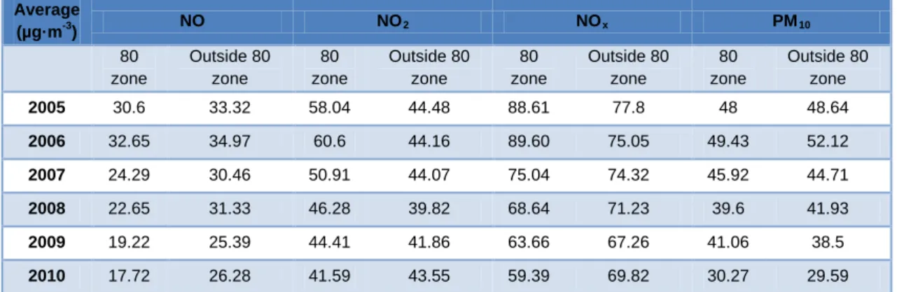
12 For all pollutants except PM10, measurements are taken every hour. The daily average was calculated from all the daily observations provided by the station. The PM10 has a daily manual sampling, so few measurements during weekends and holidays exist. The data are provided by the Monitoring Service and Air Control of the regional government. Table A1 (appendix) shows the annual average concentration for the pollutants per year and area.
The explanatory variables proposed aim to collect the pollutant source variability and its transport, sedimentation and/or reaction. Table 2 shows the explanatory variables used and their most important descriptive statistics. Traffic data includes the number of vehicles passing a specific kilometric point as close as possible to the station measuring pollution on the motorway. Measurements are taken every hour in both directions, with 48 measurements obtained daily. If we do not have these 48 measurements per day, we consider it an observation without data.
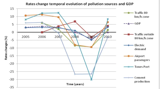
Data are provided by the Traffic Service of the regional government. As described earlier, the evolution of traffic enables us to capture the effect of the other sources that emit pollutants discussed in Table 1. Figure 3 shows the evolution of the rates of variation susceptible to pollution sources: the rate of change in the Catalonian GDP, the variation in the number of vehicles on roads inside and outside the speed limit area, the variation in electricity demand in Spain, the variation in the number of passengers carried in Barcelona airport, the tons of containers transported in the port of Barcelona, and the tons of cement produced in Catalonia. The graph shows how growth rates start to fall slightly from 2007 on. In 2009 they reach the minimum, this being between -2%
and -10%, except for maritime shipping tons and cement production, which have fallen about 25-30%. As would be expected, the slowdown of the economy reduced road traffic, electricity demand, extraction activity, the number of passengers carried in Barcelona airport, and tons transported in the port of Barcelona.
13 Table 2. Explanatory variables and descriptive statistics
The atmosphere is not watertight; there are many interactions. The meteorological variables aim to collect this variability. (a) Contaminants can be transported, so we include the average daily wind speed. (b) Pollutants are not only transported, they also undergo reaction processes. Temperature influences the reaction rate, so the average daily temperature is included. This is closely related to solar irradiance, which affects the reaction balance. (c) Water can bring a reactive change in the equilibrium or increase sedimentation, so we include relative humidity and daily rainfall. (d) Atmospheric pressure means movements of air masses ascending or descending and
Variables Description Mean Standard
deviation
Average observations per pollutant
station
Pollutants
NO2
Nitrogen dioxide daily average concentration (µg·m-3)
44.882 19.964 1807
NO
Nitric oxide daily average concentration
(µg·m-3)
26.567 29.744 1451
NOx
Nitrogen oxide daily average concentration
(µg·m-3)
70.696 44.855 1743
PM10
Particulate matter daily average concentration with less than 10 µm
(µg·m-3)
40.723 19.105 626
NO2(-1), NO(-1), NOx(-1) and PM10(-1)
One period lag variables (1 day)
80 km·h-1 speed limit
zone
Binary variable: 1 if 80 km·h-1 speed limit is
implemented. 0 otherwise
0.467 0.499 2191
Traffic Daily vehicles on both
ways 91985.6 31622.2 1500
Day Period (from 1 to 2191) 2191
Meteorological
Thermal inversion
Binary variable: 1 if there is thermal inversion the day before at 00 UTC. 0
otherwise
0.177 0.381 1809
Temperature Daily average
temperature (ºC) 16.514 6.322 1472
Relative humidity
Daily average relative
humidity (%) 66.850 11.646 1472
Precipitation Daily rainfall (mm) 1.557 5.859 1473 Wind speed Daily average wind
speed (m·s-1) 3.298 2.737 1020
Atmospheric pressure
Daily average atmospheric pressure
(hPa)
1014.8 25.418 1035
14 wind formation. At each station atmospheric pressure has been transformed into atmospheric pressure at sea level in order to establish comparisons. All the above meteorological variables except rainfall are daily averages calculated by the meteorological station. (e) One factor associated with dispersion pollutants is the thermal inversion presence. Radio-soundings have been looked at every day at Zona Universitària station (Barcelona) at 00 UTC and 12 UTC. The height of the atmosphere is analyzed up to 850 hPa (about 1500 meters above sea level). The thermal inversion is a dummy variable that takes value 1 if there is thermal inversion at 00 UTC and 0 if none is detected. The data are provided by the Meteorological Service of Catalonia (regional government).
Figure 3. Change in rates of temporal evolution of pollution sources and GDP
The variable of central policy interest is the dummy 80 km·h-1 speed limit area. It takes value 1 for stations closest to roads where the 80 km·h-1 speed limit came into force on 1 January 2008 and for stations in Barcelona city throughout the entire period of study.
The variable takes value 0 in stations for the period before the measure came into force and for those stations outside the 80 km·h-1 limit area over the entire period. For our estimations, we consider 1 January 2008 as the date the policy came into force in the affected areas. 3
3 The measure was actually introduced in December 2007, but it was introduced with no penalty for drivers who exceeded the 80 km·h-1 limit. It was from 1 January 2008 when drivers exceeding 80 km·h-1 were punishable by means of radar control. Therefore we consider 1 January 2008 as the date when the measure was effectively enforced.
15 The regression of each pollutant is accompanied by its temporal lag. When using NO and NO2 as dependent variables, we include compounds that affect the reaction balance variable and a period lag (one day). One might also expect the outcome of individuals at a particular point in time to be correlated, for example, with the proportion of diesel vehicles. Each regression includes a time variable (day).
When using differences in differences, regressions must be done with fixed effects: the correlation between the error component of station θi and the explanatory variables is different from 0. We conduct the Hausman test, and we can reject the null hypothesis at 99% significance, our fixed effects assumption being correct. Panel data errors from different stations may be correlated (contemporary correlation), and within each unit there may be temporal correlation (autocorrelation or serial correlation). Also, if the error variance is not constant, we may find heterocedasticity.
To detect autocorrelation we use the Wooldridge test. We find an autocorrelation scheme. To find heterocedasticity we use the modified Wald test for heterocedasticity.
We reject the constant variance null hypothesis. The contemporary correlation means that non-observable features in some municipalities are related to non-observable characteristics of other municipalities. One problem we have is that there is spatial correlation between pollution stations, although our pollution stations have followed a random selection. To test spatial dependence we use the Pesaran test (Pesaran, 2004). While this test introduces distortions when N is large and T is finite, our case is the opposite. Applying the test for fixed effects, we obtain spatial dependence for the four dependent variables. We use the Breusch-Pagan test, this being the null hypothesis of cross-sectional independence, which is rejected.
Once all this is taken into account, we have autocorrelation, heterocedasticity and contemporary correlation. We can solve those problems with Feasible Generalized Least Squares (FGLS) or Panel Corrected Standard Errors (PCSE). It has been demonstrated that PCSE obtain more accurate standard errors (Beck, 2001). We estimated by Ordinary Least Squares (OLS), allowing for heterocedasticity, contemporary correlation and following an AR1 autocorrelation scheme (Beck & Katz, 1995). Regarding the recommendation that the time periods should be greater than the sampling stations, it should be remembered that we have 2191 periods against 15 stations.
16 The equation we estimate for different dependent variables (NO, NO2, NOx and PM10) is the following:
Yit = β0 + β180_zoneit + β2 trafficit + β3 pollutant_lagit + β4 temperatureit + β5 humidityit + β6 rainfallit + β7 wind_speedit + β8 atmospheric_pressureit + β9 thermal_inversion_lagit
+ β10 day + θi + λt + єit
5. Results
The results of the estimations for the pollutants are reported in Table 3. To test the model’s joint significance we use the Wald test, which indicates that the variables are jointly significant at 1%. The statistic most commonly used to evaluate the model fit is the R2, which has a value between 0.67 and 0.4 depending on the pollutant. We believe this is a reasonably high explanatory capacity.
The 80 km·h-1 speed limit has a pollution-reducing effect only on NO, significant at 1%.
As regards NO2, the measure implies an increase in pollution as well as for PM10, being significant at 1%. The coming into force of the 80 km·h-1 speed limit implies a 1.93 ppm PM10 increase. As for NOx, the measure is not significant. If we take the 2007 PM10 average concentration in the speed limit area, the speed limit implies a 4.2% increase in PM10 air concentration.
Traffic is a significant variable in explaining the concentration of all pollutants except NO. The sign is positive when the variable is significant, indicating that a greater number of vehicles implies an increase in pollutant emission levels, consistent with the available evidence. An increase of 10,000 vehicles per day would mean an increase of 2.2 ppm NOx and 0.14 ppm PM10. The coefficient's significance and the expected correct sign show the importance of traffic volumes as a proxy to reflect emissions from other sources different from traffic, and how these are correlated with the economic cycle. The pollutant concentration in the previous period is significant in all regressions.
Regarding the results for the variable time (daily), the results for NOx and PM10 statistically significant but have opposite signs4; positive in the first case and negative in the second.
4 We have introduced the proportion of diesel vehicles to total vehicles per year in the province of Barcelona, but have found no explanatory power.
17 Table 3. Least-squares estimates with Panel Corrected Standard Errors
Notes: Standard errors are reported in parentheses. Each model also includes spatial and time fixed effects, and a constant term. * Statistically significant at the 10 %; ** at 5 %; and *** at 1
%.
On rainy days there is a significant reduction in PM10, NOx and NO. In the case of NO2, precipitation causes increases in atmospheric concentration. Air concentration of all pollutants increases with higher atmospheric pressure, indicating a more stable atmosphere. An increase in average wind speed implies less pollutant concentration for all pollutants. However, in the case of PM10 we could not totally rule out a positive sign;
NO NO2 NOx PM10
80 km·h-1 speed limit
-2.91835***
(0.28127)
1.81479***
(0.27074)
-0.79998 (0.55402)
1.93362***
(0.25657)
Traffic -0.0000012
(0.0000042)
0.0000641***
(0.0000043)
0.00022***
(0.000012)
0.000014***
(0.0000046)
NO2
0.79372***
(0.01310)
NO2(-1) -0.43600***
(0.01273)
0.58811***
(0.01223)
NO 0.45077***
(0.09901)
NO(-1) 0.48933***
(0.00926)
-0.24857***
(0.01115)
NOx(-1) 0.44865***
(0.01345)
PM10(-1) 0.58090***
(0.01200) Temperature -0.47648***
(0.0306)
-0.02047 (0.03547)
-1.19782***
(0.09631)
-0.08252***
(0.02769) Humidity 0.18883***
(0.01576)
-0.08589***
(0.01846)
0.20900***
(0.04766)
-0.06097***
(0.01619)
Rainfall -0.1916**
(0.03109)
0.08100**
(0.03573)
-0.18454**
(0.0900)
-0.30918***
(0.03955) Wind speed -0.32147***
(0.05186)
-0.25507***
(0.06106)
-1.66449***
(0.25318)
-0.23505***
(0.05105) Atmospheric
pressure
0.04855*
(0.02655)
0.14351***
(0.03048)
0.53597***
(0.08338)
0.35161***
(0.02775) Thermal
inversion (-1)
1.08236**
(0.45988)
-0.45564 (0.54057)
1.63791 (1.38377)
0.67928 (0.48424)
Day 0.02145***
(0.00049)
0.00072 (0.00055)
0.00748***
(0.00147)
-0.00440***
(0.00053)
R2 0.64 0.67 0.40 0.50
Nº
observations 9840 9840 9840 1898
Joint
significance 14149.52*** 8040.67*** 2700.63*** 5131.68***
18 note that PM10 is not created from an anthropogenic origin but could also be marine or coastal. In Barcelona about 4% of the PM10 concentration comes from the sea, and 44% of PM10 pollution episodes in the city come from the Sahara (Querol et al., 2001).
However, our results suggest that the wind would act as a dispersant in the Barcelona metropolitan area. The thermal inversion on the previous day at 00 UTC has a significant effect only on the NO, for which it implies an increase in atmospheric concentration. The thermal inversion presence on the previous day implies a 1.08 ppm increase in NO air concentration. The average temperature and average humidity variables have an important explanatory capacity in the model and are significant for most regressions. However, these variables affect the pollutant equilibrium equations, and the interpretation of these equations goes beyond the scope of our analysis.
Table 4 shows the results obtained from estimating the same models presented in Table 3, but omitting data obtained in the four stations in the city of Barcelona. By doing this we seek to remove from the analysis those stations that are less influenced by high-capacity roads but that are influenced by urban traffic with 50 km·h-1 speed limits. The results for NO and NO2 are basically the same with respect to the previous estimations using all stations. The only noticeable changes are that now thermal inversion is not significant for NO, and humidity has a positive effect on NO concentration and no significance on PM10 concentration.
As far as NOx is concerned, estimations excluding the stations in the city of Barcelona show a change in the policy variable. While the 80 km·h-1 speed limit was not significant with all data, when excluding the city of Barcelona the speed limit appears as significant at 1%, implying a decrease in NOx levels of 2.1% or 1.55 ppm. We have another important change involving PM10: speed limit implementation is not significant on the pollution level, whereas it did have an increasing effect in the previous estimation. The other variables keep identical sign and significance levels with the exception of the average wind speed, which has a positive sign, following the PM10
natural origin hypothesis.
19 Table 4. Least-squares estimates with Panel Corrected Standard Errors without Barcelona
data.
Notes: Standard errors are reported in parentheses. Each model also includes spatial and time fixed effects, and a constant term. * Statistically significant at the 10 %; ** at 5 %; and ***
at 1 %.
Finally, it is worth mentioning that we have conducted an additional analysis by excluding the month of August, because of its heavily seasonal conditions regarding holidays in the metropolitan area of Barcelona (and all over Spain). This leads to untypical traffic in that month. Table A2 in the Appendix shows those additional
NO NO2 NOx PM10
80 km·h-1 speed limit
-2.61999***
(0.29104)
1.32633***
(0.25450)
-1.55000***
(0.57100)
-0.34824 (0.53810)
Traffic
0.0000095*
(0.0000055)
0.0000485***
(0.0000043)
0.000183***
(0.000013)
0.000026***
(0.00001)
NO2
0.80287***
(0.01879)
NO2(-1)
-0.47117***
(0.02053)
0.60678***
(0.01332)
NO
0.40496***
(0.01056)
NO(-1)
0.50360***
(0.01411)
-0.24511***
(0.01157)
NOx(-1)
0.42031***
(0.01670)
PM10(-1)
0.54242***
(0.02160)
Temperature
-0.49990***
(0.04895)
-0.08283**
(0.03555)
-1.36046***
(0.10951)
-0.22552***
(0.05511)
Humidity
0.19273***
(0.02521)
-0.06462***
(0.01887)
0.26912***
(0.05511)
-0.03301 (0.03161)
Rainfall
-0.20271***
(0.04764)
0.07512**
(0.03545)
-0.19631**
(0.10007)
-0.34910***
(0.07644)
Wind speed
-0.33825***
(0.06672)
-0.08928 (0.05961)
-1.08907***
(0.14072)
0.22118**
(0.10558) Atmospheric
pressure
0.07725*
(0.04227)
0.15795***
(0.0303)
0.62984***
(0.09430)
0.38250***
(0.05636) Thermal
inversion (-1)
1.15610 (0.72021)
-0.25398 (0.53060)
2.1955 (1.52644)
1.35773 (0.88435)
Day
0.01949***
(0.00074)
-0.00020 (0.00054)
0.003790**
(0.01670)
-0.00628***
(0.00085)
R2 0.62 0.64 0.40 0.46
Nº
observations 6013 6013 9840 937
Joint
significance 5571.8*** 5515.78*** 1771.88*** 1405.4***
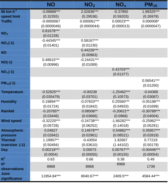
20 estimations. The estimations obtained are very similar to those presented above: the 80 km·h-1 speed limit variable always has the same sign and statistical significance for each pollutant. The most important change is in the PM10 estimation, where the temperature becomes non-significant. This also occurs in the traffic variable, which becomes only slightly significant. We can also highlight that the atmospheric pressure in NO estimation changes from significant to slightly non-significant.
6. Conclusions
This paper has analyzed the effects of reducing the speed limit to 80 km·h-1 on roads accessing the city of Barcelona. We have looked at the impact on pollution reduction of NOx and PM10. In contrast to most previous studies, this panel has relatively long periods before the measure came into force and all the periods after it came into force.
Previous speed limit experiences for 80 km·h-1 showed limited improvements in air quality. However, these experiences were studied for very short time periods or in different space locations.
The results of the empirical analysis show that the policy limiting the maximum speed to 80 km·h-1 significantly reduces NO pollution and increases NO2 pollution. For NOx, the 80 km·h-1 speed limit means a slight quality improvement, reducing pollutant air levels by 2.1% when we consider all the Barcelona metropolitan area except the city of Barcelona itself. When we consider the entire area, the measure has no effects. For PM10, the speed limit policy does not affect air quality levels when we consider the entire area, but the measure increases PM10 air levels by 4.2% when we do not consider the city of Barcelona.
Our results contradict those obtained previously by means of simulations in the same area, which associated reductions in pollutant concentration with the speed limit. When controlling for a wide range of factors that influence pollutant emissions, we find that the new speed limit has little effect – if any – on NOx. Its effects are also largely irrelevant for PM10. Traffic did consistently decrease in the years following the measure's coming into force because of the effects of the economic slowdown. This is a good proxy for the reduction in activities related to the business cycle that were important sources of emissions in the area (airport traffic, port traffic, cement …).
Therefore the economic recession has been an important factor in the decline in pollutant emissions in the area. The pronounced decrease in NOx and PM10 air
21 concentrations should not be attributed to the effects of the speed limit policy, but rather to the effects of the economic crisis.
For now, we believe that our findings provide empirical evidence that would be useful for policy makers interested in improving air quality and health in urban areas by decreasing pollutant emissions. Changing speed limits within the ranges we have evaluated may have no relevant effects on air quality, at least when compared with other policies such as congestion charging, which also reduces traffic volumes and congestion. Since the number of restrictive policies that governments can simultaneously implement is limited, choosing the best available policy maximizes the possibility of achieving the desired outcomes.
22
References
Albalate, D. & Bel, G. (2009). “What Local Policy Makers Should Know About Urban Road Charging: Lessons from Worldwide Experiences”, Public Administration Review, 69(5), 962-974.
AMMA (2008). Monitoraggio indicatori Ecopass. Prime valutazioni. City of Milan.
Baldasano, J., Gonçalves, M., Soret, A. & Jimenez-Guerrero, P. (2010). Air pollution impacts of speed limitation measures in large cities: The need for improving traffic data in a metropolitan area. Atmospheric Environment, 44 (25), 2997- 3006.
Barcelona City Council (2011). Dades bàsiques 2010. Available at http://w3.bcn.es/fitxers/mobilitat/dadesbasiques2010complert.338.pdf
Beck, N. (2001). Time-Series-Cross-Section Data: What have we learned in the past few years? Annual Review of Political Science, 4, 271-293.
Beck, N. and Katz, J. (1995). What to do (and not to do) with Time-Series Cross- Section Data. American Political Science Review, 89(3), 634-647.
Bertrand, M., Duflo, E. & Mullainathan, S. (2004). How much should we trust differences-in-differences estimates. Quarterly Journal of Economics, 119(1), 249-275.
Besley, T. & Case, A. (2000). Unnatural experiments: Estimating the incidence of Endogenous Policies. Economic Journal, 110, 672-694.
Chen, G. & Warburton, R. (2006). Do speed cameras produce net benefits? Evidence from British Columbia. Journal of Policy Analysis and Management, 25 (3), 661- 678.
Coelho, M., Farias. T. & Rouphail NM. (2005). A methodology for modelling and measuring traffic and emission performance of speed control traffic signals.
Atmospheric Environment, 39, 2367-76.
Dijkema, M., van der Zee, S., Brunekreef, B. & van Strien, R. (2008). Air quality effects of an urban highway speed limit reduction. Atmospheric Environment, 42, 9098- 9105.
EEA (2007). European Environmental Agency report Nº 2/2007: Air pollution in Europe 1990-2004 (http:/eea.europa.eu); 2007.
Eliasson, J., Hultkrantz, L., Nerhagen, L., & Rosqvist, L.S. (2009). The Stockholm congestion-charging trial 2006: overview of effects. Transportation Research A, 43 (8), 240–250.
23 Galiani, S., Gertler, P. & Schargrodsky E. (2005). Water for Life: The impact of the
privatization of water services on child mortality. Journal of Political Economy, 113, 83-120.
Gonçalves, M., Jiménez-Guerrero, P., López, E. & Baldasano, J. (2008). Air quality models sensitivity to on-road traffic speed representation: Effects on air quality of 80 km h-1 speed limit in the Barcelona Metropolitan area. Atmospheric Environment, 36, 8389-8402.
González-Marrero, R.M. & Marrero, G.A. (2011). The effect of dieselization in road transport emissions: the case of Spanish regions between 1998 and 2006.
Universidad de La Laguna, WP DT-E-2011-06
Int Panis, L., Beckx, C., Broekx, S., De Vlieger, I., Schrooten, L., Degraeuwe, B. &
Pelkmans, L. (2011). PM, NOx and CO2 emission reductions from speed management policies in Europe. Transport Policy, 18, 32-37.
Int Panis, L., Broekx, S. & Liu, R. (2006). Modelling instantaneous traffic emission and the influence of traffic speed limits, Science of the Total Environment, 371 (1-3), 270-285.
Keller, J., Andreani-Aksoyoglu, S., Tinguely, M., Flemming, J., Heldstab, J., Keller, M., Zbinden, R. & Prevot, A. (2008). The impact of reducing the màximum speed límit on motorways in Switzerland to 80 km·h-1 on emissions and peak ozone.
Environmental Modelling & Software, 23(3), 322-332.
Keuken, M.P., Jonkers, S., Wilmink, I.R. & Wesseling, J. (2010). Reduced NOx and PM10 emissions on urban motorways in The Netherlands by 80 km·h-1 speed management. Science of the Total Environment, 408(12), 2517–2526.
LAT (2006). Emissions Inventory Guidebook. Laboratory of Applied Thermodynamics (LAT), 2006. Report B710-1, Thessaloniki, Greece.
Matas, A. & Raymond, J. (2003). Demand elasticity on tolled motorways. Journal of Transportation and Statistics, 6 (2-3), 91-108.
Pesaran, M. H. (2004). General diagnostic tests for cross section dependence in panels. University of Cambridge, Faculty of Economics, Cambridge Working Papers in Economics No. 0435.
Querol, X., Alastuey, A., Rodríguez, S., Plana, F., Ruiz, C.,Cots, N., Massagué, G. &
Puig, O. (2001). PM10 and PM2.5 source apportionment in the Barcelona Metropolitan area, Catalonia, Spain. Atmospheric Environment, 35, 6407-6419.
Red Eléctrica Española (2011). El sistema eléctrico español. Disponible a:
http://www.ree.es/sistema_electrico/pdf/infosis/Inf_Sis_Elec_REE_2010.pdf
24 Rotaris, L., Danielis, R., Marcucci, E. & Massiani, J. (2010). The urban road pricing
scheme to curb pollution in Milan, Italy: Description, impacts and preliminary cost–benefit analysis assessment. Transportation Research A, 44, 359-375.
Tapio, P. (2005). Towards a theory of decoupling: degrees of decoupling in the EU and the case of road traffic in Finland between 1970 and 2001. Transport Policy, 12, 137-151.
Transport for London (2008). Impacts monitoring: Sixth annual report. London.
Wallington, T.J., Lambert, C.K. & Ruona, W.C. (forthcoming). Diesel vehicles and sustainable mobility in the U.S. Energy Policy, forthcoming
25
Appendix
Table A.1. Pollutants average concentration per years and areas
Average
(µg·m-3) NO NO2 NOx PM10
80 zone
Outside 80 zone
80 zone
Outside 80 zone
80 zone
Outside 80 zone
80 zone
Outside 80 zone
2005 30.6 33.32 58.04 44.48 88.61 77.8 48 48.64
2006 32.65 34.97 60.6 44.16 89.60 75.05 49.43 52.12
2007 24.29 30.46 50.91 44.07 75.04 74.32 45.92 44.71
2008 22.65 31.33 46.28 39.82 68.64 71.23 39.6 41.93
2009 19.22 25.39 44.41 41.86 63.66 67.26 41.06 38.5
2010 17.72 26.28 41.59 43.55 59.39 69.82 30.27 29.59
Table A.2. results from estimation excluding the month of August.
NO NO2 NOx PM10
80 km·h-1 speed limit
-3.09888***
(0.32355)
2.02836***
(0.29536)
-0.37950 (0.59203)
1.99325***
(0.26978)
Traffic -0.0000067
(0.0000046)
0.000061***
(0.0000044)
0.00023***
(0.000013)
0.000008*
(0.0000047) NO2
0.81678***
(0.01228) NO2(-1) -0.44345***
(0.01401)
0.58167***
(0.01230)
NO 0.44226***
(0.00963)
NO(-1) 0.48615***
(0.00996)
-0.24431***
(0.01089)
NOx(-1) 0.43703***
(0.01377)
PM10(-1) 0.56541***
(0.01250) Temperature -0.52825***
(0.035479)
-0.00238 (0.03701)
-1.25462***
(0.10573)
-0.04368 (0.03087) Humidity 0.19894***
(0.01724)
-0.07833***
(0.01842)
0.25560***
(0.04933)
-0.05198***
(0.01699)
Rainfall -0.20765**
(0.03446)
0.08506**
(0.03666)
-0.20621**
(0.0968)
-0.30789***
(0.04004) Wind speed -0.32220***
(0.05728)
-0.24738***
(0.06252)
-1.66282***
(0.14018)
-0.25962***
(0.05291) Atmospheric
pressure
0.04627 (0.02842)
0.14678***
(0.02961)
0.54882***
(0.08521)
0.35957***
(0.02819) Thermal
inversion (-1)
1.19907**
(0.50494)
-0.43054 (0.53610)
1.92667 (1.44102)
0.77219 (0.50179)
Day 0.00218***
(0.0054)
0.00073 (0.00055)
0.00767***
(0.00155)
-0.00446***
(0.00054)
R2 0.63 0.66 0.38 0.49
Nº
observations 8968 8968 8968
1739 Joint
significance 11954.84*** 8040.67*** 2409.5*** 4584.44***
F
UNDACIÓN DE LASC
AJAS DEA
HORROS DOCUMENTOS DE TRABAJOÚltimos números publicados
159/2000 Participación privada en la construcción y explotación de carreteras de peaje Ginés de Rus, Manuel Romero y Lourdes Trujillo
160/2000 Errores y posibles soluciones en la aplicación del Value at Risk Mariano González Sánchez
161/2000 Tax neutrality on saving assets. The spahish case before and after the tax reform Cristina Ruza y de Paz-Curbera
162/2000 Private rates of return to human capital in Spain: new evidence F. Barceinas, J. Oliver-Alonso, J.L. Raymond y J.L. Roig-Sabaté 163/2000 El control interno del riesgo. Una propuesta de sistema de límites
riesgo neutral
Mariano González Sánchez
164/2001 La evolución de las políticas de gasto de las Administraciones Públicas en los años 90 Alfonso Utrilla de la Hoz y Carmen Pérez Esparrells
165/2001 Bank cost efficiency and output specification Emili Tortosa-Ausina
166/2001 Recent trends in Spanish income distribution: A robust picture of falling income inequality Josep Oliver-Alonso, Xavier Ramos y José Luis Raymond-Bara
167/2001 Efectos redistributivos y sobre el bienestar social del tratamiento de las cargas familiares en el nuevo IRPF
Nuria Badenes Plá, Julio López Laborda, Jorge Onrubia Fernández
168/2001 The Effects of Bank Debt on Financial Structure of Small and Medium Firms in some Euro- pean Countries
Mónica Melle-Hernández
169/2001 La política de cohesión de la UE ampliada: la perspectiva de España Ismael Sanz Labrador
170/2002 Riesgo de liquidez de Mercado Mariano González Sánchez
171/2002 Los costes de administración para el afiliado en los sistemas de pensiones basados en cuentas de capitalización individual: medida y comparación internacional.
José Enrique Devesa Carpio, Rosa Rodríguez Barrera, Carlos Vidal Meliá
172/2002 La encuesta continua de presupuestos familiares (1985-1996): descripción, representatividad y propuestas de metodología para la explotación de la información de los ingresos y el gasto.
Llorenc Pou, Joaquín Alegre
173/2002 Modelos paramétricos y no paramétricos en problemas de concesión de tarjetas de credito.
Rosa Puertas, María Bonilla, Ignacio Olmeda