Solar-Driven Sorption System for Seasonal Heat Storage Under Optimal Control

Citation:Crespo, A.; Fernández, C.;

de Gracia, A.; Frazzica, A.

Solar-Driven Sorption System for Seasonal Heat Storage under Optimal Control: Study for Different Climatic Zones.Energies2022,15, 5604.

https://doi.org/10.3390/en15155604 Academic Editor: Antonio Rosato Received: 1 July 2022

Accepted: 28 July 2022 Published: 2 August 2022

Publisher’s Note:MDPI stays neutral with regard to jurisdictional claims in published maps and institutional affil- iations.

Copyright: © 2022 by the authors.

Licensee MDPI, Basel, Switzerland.

This article is an open access article distributed under the terms and conditions of the Creative Commons Attribution (CC BY) license (https://

creativecommons.org/licenses/by/

4.0/).

energies

Article

Solar-Driven Sorption System for Seasonal Heat Storage under Optimal Control: Study for Different Climatic Zones

Alicia Crespo¹, Cèsar Fernández¹, Alvaro de Gracia²and Andrea Frazzica^3,*

1 GREiA Research Group, University of Lleida, Pere de Cabrera s/n, 25001 Lleida, Spain;

[email protected] (A.C.); [email protected] (C.F.)

2 IT4S Research Group, Universitat de Lleida, Pere de Cabrera s/n, 25001 Lleida, Spain; [email protected]

3 Institito di Tecnologie Avanzate per l’Energia “Nicola Giordano”, CNR-ITAE, 98126 Messina, Italy

* Correspondence: [email protected]

Abstract:Solar thermal energy coupled to a seasonal sorption storage system stands as an alternative to fossil fuels to supply residential thermal energy demand in climates where solar energy availability is high in summer and low in winter, matching with a high space heating demand. Sorption storage systems usually have a high dependency on weather conditions (ambient temperature and solar irradiation). Therefore, in this study, the technical performance of a solar-driven seasonal sorption storage system, using an innovative composite sorbent and water as working fluid, was studied under three European climates, represented by: Paris, Munich, and Stockholm. All scenarios analyses were simulation-based under optimal system control, which allowed to maximize the system competitiveness by minimizing the system operational costs. The optimal scenarios profit from just 91, 82 and 76% of the total sorption system capacity, for Paris, Munich, and Stockholm, respectively.

That means that an optimal control can identify the optimal sorption storage size for each location and avoid oversizing in future systems, which furthermore involves higher investment costs. The best coefficient of performance was obtained for Stockholm (0.31), despite having the coldest climate.

The sorption system was able to work at minimum temperatures of−15^◦C, showing independence from ambient temperature during its discharge. In conclusion, a seasonal sorption system based on selective water materials is suitable to be integrated into a single-family house in climates of central and northern Europe as long as an optimal control based on weather conditions, thermal demand, and system state is considered.

Keywords: water-based sorption storage; seasonal storage; simulations; control optimization;

climatic zones

1. Introduction

The objective of the Paris Agreement reached at COP21 [1] was to limit global warming

“well-below 2 ^◦C” above pre-industrial levels. To reach this challenging goal, a global energy transition where clean energies take a centre stage is fundamental. According to the International Energy Agency (IEA) [2], heat is the largest energy end-use, accounting for half of the global final energy consumption. Focusing on the residential sector, the thermal demand accounts for 46% of the global heat consumption [3]. Renewable heat sources, such as solar energy, could contribute to supply a large percentage of that global heat consumption, leading us to a decarbonize energy matrix. Nevertheless, modern renewables account for only 11% of global heat supply today [2]. In particular, solar collectors coupled to seasonal thermal energy storage makes it possible to store solar heat during summer and release it in winter, when the solar resource availability is low and the space heating demands in the households are high.

Yang et al. [4] reviewed six types (see Figure1) of seasonal thermal energy storage systems from a techno-economic perspective. According to the authors, latent and ther- mochemical storage exhibit the best technical performance. Latent heat storage can be

Energies2022,15, 5604. https://doi.org/10.3390/en15155604 https://www.mdpi.com/journal/energies

Energies2022,15, 5604 2 of 23

considered a good candidate due to its high energy density and its ability to supply heat at a nearly constant temperature. Nevertheless, it presents several disadvantages, among which stand out the lack of thermal stability, the potential degradation [4], and the thermal losses between summer and winter seasons. Thermochemical storage based on the sorption process stands as a very promising solution for seasonal TES since it presents zero thermal losses during the storage period, which is a crucial requirement for long-term seasonal storage. Furthermore, sorption storage also presents high energy densities at material level.

Nevertheless, thermochemical storage requires further research at the material, system, and operational level.

Energies 2022, 15, x FOR PEER REVIEW 2 of 23

Yang et al. [4] reviewed six types (see Figure 1) of seasonal thermal energy storage systems from a techno-economic perspective. According to the authors, latent and ther- mochemical storage exhibit the best technical performance. Latent heat storage can be considered a good candidate due to its high energy density and its ability to supply heat at a nearly constant temperature. Nevertheless, it presents several disadvantages, among which stand out the lack of thermal stability, the potential degradation [4], and the ther- mal losses between summer and winter seasons. Thermochemical storage based on the sorption process stands as a very promising solution for seasonal TES since it presents zero thermal losses during the storage period, which is a crucial requirement for long- term seasonal storage. Furthermore, sorption storage also presents high energy densities at material level. Nevertheless, thermochemical storage requires further research at the material, system, and operational level.

Figure 1. Schematic representation of the nodes of the TES [4].

The sorption storage process is based on the reaction between a sorbate, sometimes referred to as working fluid (e.g., water, ammonia, alcohols) and a sorbent, which can be either a solid or a liquid solution. The interaction between the two components is either physical or through weak chemical reactions [5]. For this reason, sorption processes are suitable for residential applications since the reversible reaction can be driven by low- medium charging temperatures (i.e., 80–120 °C) [6], which can be provided by commercial non-concentrating solar thermal technologies.

Several authors have already studied ammonia-based sorption storage systems for space heating applications [7–9]. This type of sorption systems has the advantages of high- operation pressure and low freezing point of liquid ammonia compared to water-based sorption storage [10]. Nevertheless, the toxicity of ammonia can hinder its commercial implementation in the residential sector. Sorption TES based on a water sorbent is a more environmentally friendly solution for households. Some authors have studied its thermal performance for heating generation at a pilot scale [11–15]. Most of the studies analysed or optimized system parameters such as outlet temperature, mass transfer, or energy den- sity under well-defined testing conditions. Nevertheless, an extrapolation from the proto- types or small-scale systems to full-scale systems coupled to the dynamics of a dwelling thermal demand and weather conditions requires attention from the scientific commu- nity. Sorption storage systems require a low temperature heat source (above 0 °C for wa- ter-based ones) to assist the evaporator. During intermediate season or warm winter days, ambient air can be used as heat source. In summer, ambient air can also be used as heat sink by the condenser. Moreover, when solar heat is also used as heat source, the system dependency on weather conditions is higher. Therefore, to really understand the impact of weather conditions and optimize the thermal performance of sorption heat storage sys- tems at a real scale, a study of the system coupled to a dwelling thermal demand subjected to different climates must be carried out. Few studies analysed the impact of different climatic conditions on seasonal sorption systems. Ma et al. [16] studied the feasibility of using sensible, latent, and thermochemical storage technologies to supply the space heat-

Figure 1.Schematic representation of the nodes of the TES [4].

The sorption storage process is based on the reaction between a sorbate, sometimes referred to as working fluid (e.g., water, ammonia, alcohols) and a sorbent, which can be either a solid or a liquid solution. The interaction between the two components is either physical or through weak chemical reactions [5]. For this reason, sorption processes are suitable for residential applications since the reversible reaction can be driven by low- medium charging temperatures (i.e., 80–120^◦C) [6], which can be provided by commercial non-concentrating solar thermal technologies.

Several authors have already studied ammonia-based sorption storage systems for space heating applications [7–9]. This type of sorption systems has the advantages of high- operation pressure and low freezing point of liquid ammonia compared to water-based sorption storage [10]. Nevertheless, the toxicity of ammonia can hinder its commercial implementation in the residential sector. Sorption TES based on a water sorbent is a more environmentally friendly solution for households. Some authors have studied its thermal performance for heating generation at a pilot scale [11–15]. Most of the studies analysed or optimized system parameters such as outlet temperature, mass transfer, or energy density under well-defined testing conditions. Nevertheless, an extrapolation from the prototypes or small-scale systems to full-scale systems coupled to the dynamics of a dwelling thermal demand and weather conditions requires attention from the scientific community. Sorption storage systems require a low temperature heat source (above 0^◦C for water-based ones) to assist the evaporator. During intermediate season or warm winter days, ambient air can be used as heat source. In summer, ambient air can also be used as heat sink by the condenser. Moreover, when solar heat is also used as heat source, the system dependency on weather conditions is higher. Therefore, to really understand the impact of weather conditions and optimize the thermal performance of sorption heat storage systems at a real scale, a study of the system coupled to a dwelling thermal demand subjected to different climates must be carried out. Few studies analysed the impact of different climatic conditions on seasonal sorption systems. Ma et al. [16] studied the feasibility of using sensible, latent, and thermochemical storage technologies to supply the space heating (SH) and domestic hot water (DHW) demand of domestic dwellings in eight representative cities of the UK. Nevertheless, the authors did not deepen into the performance of the thermochemical storage system. Engel et al. [17] performed a detailed simulation of a solar-driven water-based sorption storage system. The solar fraction of the sorption system was analysed for different locations under different building load profiles

Energies2022,15, 5604 3 of 23

(15, 30, 60 and 100 kWh/m³). All simulations were performed with one set of parameters and system dimensions. However, the control settings were not optimal for all the locations and heat demands. Indeed, the authors reported that for some locations, the sorption storages were considerably oversized and that it could have been avoided by adjusting the control strategy. On a yearly basis, Mlakar et al. [18] simulated the performance of a thermochemical storage that supplied space heating to a building located in two Slovenian locations: Ljubljana and Portorož. The software tools: TRNSYS and MS Excel, were used to simulate the system. The results showed that the simulation was highly dependent on the climatic conditions of each geographical location. Furthermore, the study showed that thermochemical storage can achieve 100% of coverage for heat demand of a building.

Jiang et al. [7] analysed a hybrid ammonia-based sorption seasonal storage driven by PVT collectors under three different severe cold regions. The authors concluded that the hybrid technology could be promising to solve the heating issues in severe cold regions during winter. Frazzica et al. [19] proposed a new unified methodology for the optimization of the seasonal sorption storage sizing, depending on building constraints, weather conditions, and solar thermal technologies. The method was based on energy balance considerations and climatic analysis, thus providing a tool for the sizing but not focusing on any optimized operation of the technology.

As N’Tsoukpoe et al. [20] reported, seasonal sorption storage systems are subjected to significant sensible thermal losses, which in turn impact in the COP of the system, which represents the ratio between the energy discharged in winter to the energy stored in summer. An optimal control of the system can contribute to minimize the heat losses between two consecutive charges and discharges by identifying which system states and weather conditions benefit its performance. Furthermore, other studies [18] have already proved the dependency of sorption storage systems on climatic conditions. Therefore, in this study, the performance of a seasonal sorption storage composed by an innovative asymmetric heat exchanger (reactor) [21] filled by a novel selective water sorbent (SWS) [22]

was studied under different climatic conditions. Moreover, as Engel et al. [17] reported, adjusting the control strategy for each location can avoid oversizing. Nevertheless, to the authors knowledge, the analysis of a solar-driven sorption seasonal sorption system subjected to different climate conditions, each of them operated under detailed optimal control, has not been studied before. Hence, in this study, in addition to analysing the impact of different weather conditions on the thermal performance of a sorption thermal energy storage (STES) system, the optimal control scenario for each location was identified and analysed. The seasonal energy system which supplied SH and DHW to a single-family house was studied through numerical simulations under three different locations: Paris, Munich, and Stockholm. The system was operated with a rule-based control (RBC) strategy, which was optimized for the corresponding thermal demand, solar irradiation, ambient temperature, and system conditions of each location. The authors of the present study are aware of the actual limitations of long-term solar heat storage for household application.

Precisely for that, we think that further research, especially in the design optimization, system integration, and control, is necessary. The present study will help to open a better scenario with respect to the integration of seasonal sorption systems into households.

This study is divided as follows. Section2describes the methodology followed. It in- cludes a description of the system and its operation and a description of the numerical mod- els. An explanation of the three case studies and their control optimization methodology is also included in Section2. Sections3and4present the results and conclusions, respectively.

2. Methodology

2.1. Solar-Driven Seasonal Sorption System

In this study, the impact of climatic conditions on the performance of a solar-driven seasonal water-based sorption system that supplied domestic hot water (DHW) and space heating (SH) to a single-family house is analysed. Evacuated tube collectors supplied heat to either a stratified water tank, a seasonal sorption storage system, or a low temperature

Energies2022,15, 5604 4 of 23

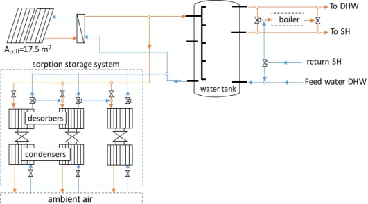
heat source (LTHS), depending on the season, solar irradiation, ambient temperature, and the state variables. During the summer season (from April to end of September), solar heat with high enthalpy was used to charge the sorption storage system at regeneration temperatures around 90 ^◦C. The sorption storage was composed by 20 modules of a composite material which consisted of LiCl embedded in a Silica gel matrix [22] (known as selective water sorbent (SWS)). The sorption storage used ambient air as environmental sink to the condenser during its charging process. In addition to charge the sorption modules in summer, solar heat at lower enthalpy was used to charge the stratified water tank for DHW application (65^◦C), and to a lower extent for SH during the intermediate season. DHW and SH were supplied from the upper and middle part of the water tank, respectively (see Figure2), when needed. A back-up gas boiler assisted the system when the temperature in the stratified water tank was below the corresponding set point.

Energies 2022, 15, x FOR PEER REVIEW 4 of 23

2. Methodology

2.1. Solar-Driven Seasonal Sorption System

In this study, the impact of climatic conditions on the performance of a solar-driven seasonal water-based sorption system that supplied domestic hot water (DHW) and space heating (SH) to a single-family house is analysed. Evacuated tube collectors supplied heat to either a stratified water tank, a seasonal sorption storage system, or a low temperature heat source (LTHS), depending on the season, solar irradiation, ambient temperature, and the state variables. During the summer season (from April to end of September), solar heat with high enthalpy was used to charge the sorption storage system at regeneration tem- peratures around 90 °C. The sorption storage was composed by 20 modules of a composite material which consisted of LiCl embedded in a Silica gel matrix [22] (known as selective water sorbent (SWS)). The sorption storage used ambient air as environmental sink to the condenser during its charging process. In addition to charge the sorption modules in sum- mer, solar heat at lower enthalpy was used to charge the stratified water tank for DHW application (65 °C), and to a lower extent for SH during the intermediate season. DHW and SH were supplied from the upper and middle part of the water tank, respectively (see Figure 2), when needed. A back-up gas boiler assisted the system when the temperature in the stratified water tank was below the corresponding set point.

Figure 2. Schematic of the system for summer configuration.

During winter (from October to end of March), the solar energy availability was low and the SH heating demand was high. Therefore, when there was SH demand and the middle part of the water tank was below the set-point, heat of sorption was discharged from the sorption modules to the stratified water tank. The sorption storage was dis- charged at a composite temperature of 35 °C. The SH demand set-point was dependent of the ambient temperature, according the floor SH distribution system [23]. Due to the working cycle of the selected composite material, radiant floor heating was selected, which works at supply temperature ranging from 25 to 35 °C, depending on the energy

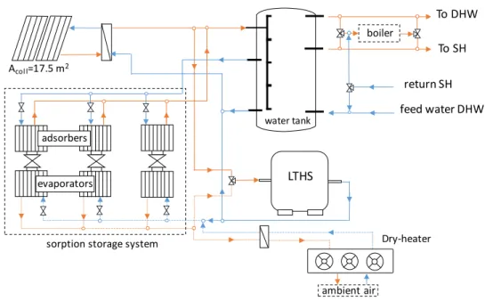
Water-based sorption storage systems require a low temperature heat source that supplies heat above 0 °C (from 5 to 15 °C in this case) to the evaporator during the dis- charging process. In the proposed system, to avoid full dependency of the sorption system to the ambient temperature, a low temperature heat source charged by solar energy at low enthalpy was implemented (see Figure 3). Additionally, if the ambient temperatures where high enough, ambient heat was used to assist the evaporator.

To DHW

To SH

sorption storage system

ambient air

boiler

return SH Feed water DHW Acol l=17.5 m²

water tank

desorbers

condensers

Figure 2.Schematic of the system for summer configuration.

During winter (from October to end of March), the solar energy availability was low and the SH heating demand was high. Therefore, when there was SH demand and the middle part of the water tank was below the set-point, heat of sorption was discharged from the sorption modules to the stratified water tank. The sorption storage was discharged at a composite temperature of 35^◦C. The SH demand set-point was dependent of the ambient temperature, according the floor SH distribution system [23]. Due to the working cycle of the selected composite material, radiant floor heating was selected, which works at supply temperature ranging from 25 to 35^◦C, depending on the energy efficiency of the building’s envelope and outdoor ambient temperature.

Water-based sorption storage systems require a low temperature heat source that supplies heat above 0^◦C (from 5 to 15 ^◦C in this case) to the evaporator during the discharging process. In the proposed system, to avoid full dependency of the sorption system to the ambient temperature, a low temperature heat source charged by solar energy at low enthalpy was implemented (see Figure3). Additionally, if the ambient temperatures where high enough, ambient heat was used to assist the evaporator.

EnergiesEnergies 2022, 15, x FOR PEER REVIEW 2022,15, 5604 5 of 23 5 of 23

Figure 3. Schematic of the system for winter configuration.

As happened in summer, during winter days with relatively high solar irradiation the stratified water tank was charged with solar heat to supply DHW and SH needs. SH demand was supplied directly by the stratified tank, with assistance from the back-up boiler or working in close loop when the temperatures in the middle part of the water tank were below 20 °C (lower than the SH return temperature). When the gas boiler was required by both DHW and SH, the DHW was prioritized, which means that, during the corresponding time period (usually 15 min), the system was not accomplishing the user comfort.

2.2. System Simulation

Numerical models and performance maps implemented in Python [24] were used to simulate the thermal performance of the different subcomponents of the system. Once all models described below were implemented, their interconnection and coupling with the transient weather data and thermal demand was carried out also in Python. A time-step of 15 min was used for the simulations. The same subsystems design parameters (size, mass flow rate, etc.), which were derived from the technical report of a European project [25], were considered to analyse the different climatic locations.

Solar collectors

A 17.5 m

solar field composed by evacuated tube collectors [26] was used in the simulations. The generic equation of the thermal performance of a solar collector pre- sented by Duffie and Beckman [27] can be expressed based on the collector overall effi- ciency (η

), as shown in Equations (1) and (2):

𝐼𝐴𝑀 𝐸_𝐺 𝐴_𝑐𝑜𝑙 𝜂_{𝑜𝑣𝑒𝑟𝑎𝑙𝑙} = 𝑚˙_𝑐𝑜𝑙 𝐶_𝑝(𝑇_{𝑜𝑢𝑡,𝑐𝑜𝑙}− 𝑇_{𝑖𝑛,𝑐𝑜𝑙})

(1)

𝐸𝐺 − 𝑎₂^{(𝑇𝑎𝑣𝑔,𝑐𝑜𝑙−𝑇𝑎𝑚𝑏)}

𝐸𝐺 2

(2)

where IAM is the incidence angle modifier, E

is the solar global irradiation in the titled surface, A

is the collector area,

is the collector mass flow rate,

, T

and

are the outlet, inlet, and average collector temperatures, respectively, a

is the col- lector optical efficiency and a

and a

are the first and second order collector efficiencies, respectively. Water-glycol with a specific heat (C

) of 3.9 kJ/kg·K was considered as HTF in the simulations. The optimal and thermal properties of the collector are shown in Table 1.

Acol l=17.5 m²

water tank

LTHS

sorption storage system

To DHW To SH boiler

return SH feed water DHW

Dry-heater

ambient air adsorbers

evaporators

Figure 3.Schematic of the system for winter configuration.

As happened in summer, during winter days with relatively high solar irradiation the stratified water tank was charged with solar heat to supply DHW and SH needs. SH demand was supplied directly by the stratified tank, with assistance from the back-up boiler or working in close loop when the temperatures in the middle part of the water tank were below 20^◦C (lower than the SH return temperature). When the gas boiler was required by both DHW and SH, the DHW was prioritized, which means that, during the corresponding time period (usually 15 min), the system was not accomplishing the user comfort.

2.2. System Simulation

Numerical models and performance maps implemented in Python [24] were used to simulate the thermal performance of the different subcomponents of the system. Once all models described below were implemented, their interconnection and coupling with the transient weather data and thermal demand was carried out also in Python. A time-step of 15 min was used for the simulations. The same subsystems design parameters (size, mass flow rate, etc.), which were derived from the technical report of a European project [25], were considered to analyse the different climatic locations.

Solar collectors

A 17.5 m² solar field composed by evacuated tube collectors [26] was used in the simulations. The generic equation of the thermal performance of a solar collector presented by Duffie and Beckman [27] can be expressed based on the collector overall efficiency (ηoverall), as shown in Equations (1) and (2):

I AM E_GA_colη_overall =m^._colCp(T_out,col−T_in,col) (1)

η_overall =a0−a1

Tavg,col−Tamb

EG

−a2

T_avg,col−T_amb EG

2

(2) whereIAMis the incidence angle modifier,EGis the solar global irradiation in the titled surface,Acolis the collector area,m^.colis the collector mass flow rate,Tout,col,Tin,coland T_avg,col are the outlet, inlet, and average collector temperatures, respectively, a₀ is the collector optical efficiency anda₁anda₂are the first and second order collector efficiencies, respectively. Water-glycol with a specific heat (Cp) of 3.9 kJ/kg·K was considered as HTF in the simulations. The optimal and thermal properties of the collector are shown in Table1.

Energies2022,15, 5604 6 of 23

Table 1.Optical and thermal properties of the solar collector used in the simulations.

Parameter Value Parameter Value

a₀ 0.559 [28] Mass flow range (kg/h) 300–1000

a₁(W/m²K) 1.485 [28] Diffuse IAM 1.314 [28]

a₂(W/m²K²) 0.002 [28] Maximum pressure (bar) 10 [29]

The evacuated tube collector model was validated against results reported by Ay- ompe et al. [30]. The deviation between the reference and the present model was lower than 1% in terms of the collector outlet temperature average relative error.

Stratified water tank

A constant volume stratified water tank was used in the simulations to store solar heat and supply it for DHW and SH. A 1D numerical model which considered thermal losses to the ambient, conduction between adjacent nodes, and mass exchange between nodes was used. The model was based on the finite control volume method, i.e., every control volume had uniform thermal properties. The set of equations, solved with an explicit scheme, used to model the heat transfer in the water tank were presented by Rodriguez-Hidalgo et al. [31].

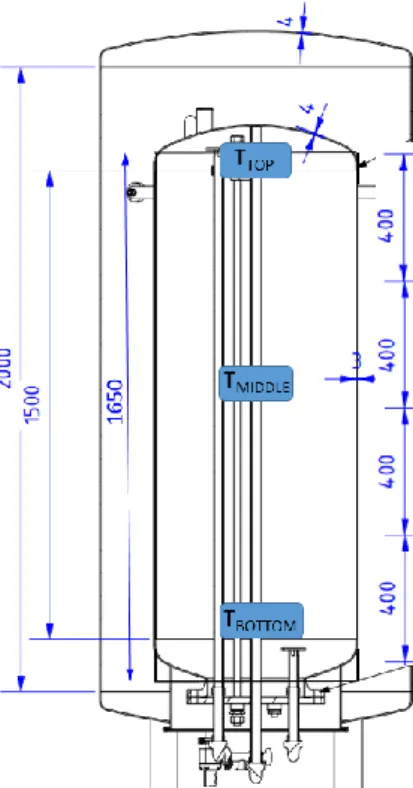
A sketch of the stratified tank used in the simulation is shown in Figure4. The original water tank (as shown in Figure4) did not have a perfect cylindrical shape. An equivalent height considering a perfect cylindrical shape was considered to allow for a structured grid in the discretization of the domain. The model, simulated using 33 control volumes (nodes), was validated against experiments performed at the laboratory of GREiA at the University of Lleida. For the validation, just five nodes along the tank were considered, obtaining an average error of 2.1%. More information about the set-up and the water tank can be found at [32].

Energies 2022, 15, x FOR PEER REVIEW 6 of 23

Table 1. Optical and thermal properties of the solar collector used in the simulations.

Parameter Value Parameter Value

a

0.559 [28] Mass flow range (kg/h) 300–1000 a

(W/m

K) 1.485 [28] Diffuse IAM 1.314 [28]

a

(W/m

K

) 0.002 [28] Maximum pressure (bar) 10 [29]

The evacuated tube collector model was validated against results reported by Ayompe et al. [30]. The deviation between the reference and the present model was lower than 1% in terms of the collector outlet temperature average relative error.

Stratified water tank

A constant volume stratified water tank was used in the simulations to store solar heat and supply it for DHW and SH. A 1D numerical model which considered thermal losses to the ambient, conduction between adjacent nodes, and mass exchange between nodes was used. The model was based on the finite control volume method, i.e., every control volume had uniform thermal properties. The set of equations, solved with an ex- plicit scheme, used to model the heat transfer in the water tank were presented by Rodri- guez-Hidalgo et al. [31].

A sketch of the stratified tank used in the simulation is shown in Figure 4. The origi- nal water tank (as shown in Figure 4) did not have a perfect cylindrical shape. An equiv- alent height considering a perfect cylindrical shape was considered to allow for a struc- tured grid in the discretization of the domain. The model, simulated using 33 control vol- umes (nodes), was validated against experiments performed at the laboratory of GREiA at the University of Lleida. For the validation, just five nodes along the tank were consid- ered, obtaining an average error of 2.1%. More information about the set-up and the water tank can be found at [32].

Figure 4. Sketch of the stratified tank [33] used in the simulations.

The control policy of the system required the instant temperature values at the top and middle part of the water tank, which corresponded to the regions intended for DHW and SH, respectively. That means that, out of the 33 control volumes, just 3 of them (sim- ulating 3 sensors) located at the top, middle, and bottom part of the stratified tank were

The control policy of the system required the instant temperature values at the top and middle part of the water tank, which corresponded to the regions intended for DHW and SH, respectively. That means that, out of the 33 control volumes, just 3 of them (simulating

Energies2022,15, 5604 7 of 23

3 sensors) located at the top, middle, and bottom part of the stratified tank were used in the simulations as control parameters. The parameters of the stratified water tank used in the simulations are presented in Table2.

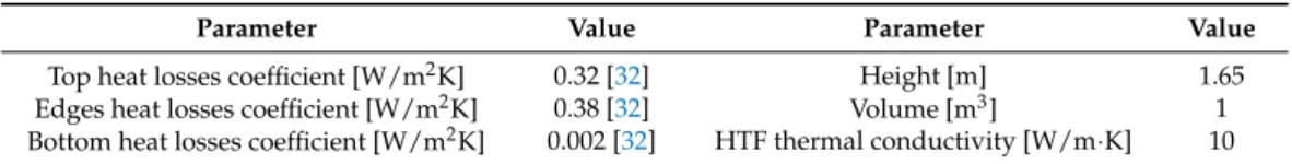
Table 2.Parameters of the stratified water tank used in the simulations.

Parameter Value Parameter Value

Top heat losses coefficient [W/m²K] 0.32 [32] Height [m] 1.65

Edges heat losses coefficient [W/m²K] 0.38 [32] Volume [m³] 1

Bottom heat losses coefficient [W/m²K] 0.002 [32] HTF thermal conductivity [W/m·K] 10

Sorption storage tank

Some studies tested prototypes of sorption reactors at laboratory or pilot-scale for TES applications using solid pure adsorbents or composite materials [12–15,34]. Scaling up the reactors from laboratory scale or pilot scale to real scale entails design, manufacturing, and testing challenges. To the authors knowledge, just one study [12] analysed a closed sorption storage system at real-scale for household SH application using composite materials, as the one presented in this study. Studies about the thermal performance of real-scale reactors of both open and closed systems is missing in the literature. For this reason, Hu et al. [35]

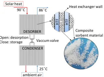
presented a set of ratios to scale up an open zeolite sorption TES from a pilot to full-scale, which theoretically ensured similar geometry, dynamics, sorption-kinetics, and thermal performance. In this study, the thermal performance of the closed sorption TES system under study was obtained from the scaling up of experimental tests. The experimental measurements of a novel lab-scale adsorber (asymmetric plate heat exchanger) reported by Mikhaeil et al. [21] together with the kinetic characterization [36] of the water adsorbent material used in this study (LiCl/silica gel) were scaled up to obtain the performance maps of 100 kg SWS sorption module. A detailed sketch of a sorption module is shown in Figure5(temperatures correspond to charging process).

Energies 2022, 15, x FOR PEER REVIEW 7 of 23

used in the simulations as control parameters. The parameters of the stratified water tank used in the simulations are presented in Table 2.

Table 2. Parameters of the stratified water tank used in the simulations.

Parameter Value Parameter Value

Top heat losses coefficient [W/m²K] 0.32 [32] Height [m] 1.65 Edges heat losses coefficient [W/m²K] 0.38 [32] Volume [m³] 1 Bottom heat losses coefficient [W/m²K] 0.002 [32] HTF thermal conductivity [W/m·K] 10 Sorption storage tank

Some studies tested prototypes of sorption reactors at laboratory or pilot-scale for TES applications using solid pure adsorbents or composite materials [12–15,34]. Scaling up the reactors from laboratory scale or pilot scale to real scale entails design, manufac- turing, and testing challenges. To the authors knowledge, just one study [12] analysed a closed sorption storage system at real-scale for household SH application using composite materials, as the one presented in this study. Studies about the thermal performance of real-scale reactors of both open and closed systems is missing in the literature. For this reason, Hu et al. [35] presented a set of ratios to scale up an open zeolite sorption TES from a pilot to full-scale, which theoretically ensured similar geometry, dynamics, sorption- kinetics, and thermal performance. In this study, the thermal performance of the closed sorption TES system under study was obtained from the scaling up of experimental tests.

The experimental measurements of a novel lab-scale adsorber (asymmetric plate heat ex- changer) reported by Mikhaeil et al. [21] together with the kinetic characterization [36] of the water adsorbent material used in this study (LiCl/silica gel) were scaled up to obtain the performance maps of 100 kg SWS sorption module. A detailed sketch of a sorption module is shown in Figure 5 (temperatures correspond to charging process).

Figure 5. Adsorption heat exchanger in detail.

The performance maps (see Figure 6) provided the charging and discharging power as a function of the adsorber inlet temperature and the condenser or evaporator inlet tem- perature, respectively. The following mass flow rates were used to obtain the performance maps: 0.2 kg/s in the adsorber, 0.25 kg/s in the condenser, 0.166 kg/s in the evaporator.

The calculated maximum stored energy corresponds to 110 MJ per module.

CONDENSER

ambient air DESORBER

25 ͦC 86 ͦC 90 ͦC

Solar heat

Vaccum valve Close: storage

HTF HTF

Open: desorption

Composite sorbent material Heat exchanger wall

Figure 5.Adsorption heat exchanger in detail.

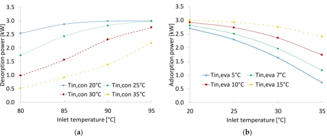
The performance maps (see Figure6) provided the charging and discharging power as a function of the adsorber inlet temperature and the condenser or evaporator inlet tem- perature, respectively. The following mass flow rates were used to obtain the performance maps: 0.2 kg/s in the adsorber, 0.25 kg/s in the condenser, 0.166 kg/s in the evaporator.

The calculated maximum stored energy corresponds to 110 MJ per module.

Energies2022,15, 5604 8 of 23

Energies 2022, 15, x FOR PEER REVIEW 8 of 23

(a) (b)

Figure 6. Charging (a) and discharging (b) performance map of a 100 kg sorption module.

The performance of a sorption system is dependent on the ambient thermal losses between two consecutive charges or discharges. The higher the thermal losses, the more sensible heat will be consumed by the module to reach the regeneration or adsorption temperature again, which negatively impacts on the COP (i.e., the round-trip efficiency of the TES). To calculate the thermal losses, each sorption module was assumed as a lumped system, representing the composite material, the metal heat exchanger, and the HTF. The temperature difference between the module temperature, considered uniform for all the system, and the ambient temperature was the driving force of the heat losses. The sorption storage was assumed to be in a non-heated area of the house or even buried underground.

Thus, a constant ambient temperature of 15 °C and 21 °C for winter and summer, respec- tively, was assumed. In spite of assuming an ambient temperature of 15 °C during winter, a low temperature heat source is required. Otherwise, due to the relatively continuously evaporator heat demand, since the system is located in a closed space, the surrounding temperature would drop down, cooling down the ambient air and thus not being able to provide ambient heat anymore.

Furthermore, a standard insulation of 5 cm of polyurethane, with a thermal conduc- tivity of 0.03 W/m·K, was considered. Under this scenario, the decline of the sorption mod- ule was calculated by an exponential decay function, depending on the heat transfer co- efficient, calculated based on the natural convection and insulation heat transfer coeffi- cient, an equivalent heat capacity, the total mass of the module, and its external heat trans- fer area.

Auxiliary elements

The auxiliary subcomponents, the gas boiler, the dry heater, and a buffer water tank (low temperature heat storage) were modelled using state-of-the-art numerical models.

The gas boiler was modelled based on the mathematical description used in the type 122 of TRNSYS 18 Documentation [37]. The thermal power (Q) delivered by the dry heater was represented by Equation (3): the equality between the temperature gradient between the inlet and the outlet HTF (water-glycol) temperatures (T

and T

) and the Fou-

thermal transmittance of the dry heater heat exchanger per surface area. The UA of the dry heater indicated by the manufacturer [39] under its operating conditions was 320 W/m

K. The maximum thermal power of the boiler and the dry heater considered in the simulations was 9 and 2.75 kW, respectively.

𝑄 = 𝑚 ˙ 𝐶_{𝑝,𝐻𝑇𝐹}(𝑇_{𝑜𝑢𝑡,𝐻𝑇𝐹}− 𝑇_{𝑖𝑛,𝐻𝑇𝐹}) = 𝑈𝐴_{𝑑𝑟𝑦𝑐𝑜𝑜𝑙𝑒𝑟}(𝑇_𝑎𝑚𝑏− 𝑇_{𝑎𝑣𝑔,𝑎𝑖𝑟})

(3)

0.5 1.0 1.5 2.0 2.5 3.0 3.5

80 85 90 95

Desorption power [kW]

Inlet temperature [°C]

Tin,con 20°C Tin,con 25°C Tin,con 30°C Tin,con 35°C

0.0 0.5 1.0 1.5 2.0 2.5 3.0 3.5

20 25 30 35

Adsorption power [kW]

Inlet temperature [°C]

Tin,eva 5°C Tin,eva 7°C Tin,eva 10°C Tin,eva 15°C

Figure 6.Charging (a) and discharging (b) performance map of a 100 kg sorption module.

The performance of a sorption system is dependent on the ambient thermal losses between two consecutive charges or discharges. The higher the thermal losses, the more sensible heat will be consumed by the module to reach the regeneration or adsorption temperature again, which negatively impacts on the COP (i.e., the round-trip efficiency of the TES). To calculate the thermal losses, each sorption module was assumed as a lumped system, representing the composite material, the metal heat exchanger, and the HTF. The temperature difference between the module temperature, considered uniform for all the system, and the ambient temperature was the driving force of the heat losses.

The sorption storage was assumed to be in a non-heated area of the house or even buried underground. Thus, a constant ambient temperature of 15^◦C and 21^◦C for winter and summer, respectively, was assumed. In spite of assuming an ambient temperature of 15^◦C during winter, a low temperature heat source is required. Otherwise, due to the relatively continuously evaporator heat demand, since the system is located in a closed space, the surrounding temperature would drop down, cooling down the ambient air and thus not being able to provide ambient heat anymore.

Furthermore, a standard insulation of 5 cm of polyurethane, with a thermal conductiv- ity of 0.03 W/m·K, was considered. Under this scenario, the decline of the sorption module was calculated by an exponential decay function, depending on the heat transfer coefficient, calculated based on the natural convection and insulation heat transfer coefficient, an equivalent heat capacity, the total mass of the module, and its external heat transfer area.

Auxiliary elements

The auxiliary subcomponents, the gas boiler, the dry heater, and a buffer water tank (low temperature heat storage) were modelled using state-of-the-art numerical models.

The gas boiler was modelled based on the mathematical description used in the type 122 of TRNSYS 18 Documentation [37]. The thermal power (Q) delivered by the dry heater was represented by Equation (3): the equality between the temperature gradient between the inlet and the outlet HTF (water-glycol) temperatures (T_out,HTFandT_in,HTF) and the Fourier’s law of heat conduction [38]. The UA value, shown in Equation (3), represents the thermal transmittance of the dry heater heat exchanger per surface area. The UA of the dry heater indicated by the manufacturer [39] under its operating conditions was 320 W/m²K. The maximum thermal power of the boiler and the dry heater considered in the simulations was 9 and 2.75 kW, respectively.

Q=m C^. p,HTF(Tout,HTF−T_in,HTF) =U A_drycooler T_amb−T_avg,air

(3) The water buffer tank that assisted the evaporator during the discharge of the sorp- tion storage was modelled assuming one single control volume of 0.39 m³with uniform

Energies2022,15, 5604 9 of 23

temperature. Thermal losses to the ambient were neglected due to its short-term use (some hours).

2.3. Control Description

The system could select between 43 operational modes (described in AppendixA), which consisted in the combination of the operational modes of the solar field, stratified water tank (i.e., combi-tank), sorption storage tank, boiler, and SH supply mode explained in Section2.1and presented in Table3. The operation of the system was controlled by an RBC policy implemented also in Python by the authors of this study. The RBC policy selected an operational mode based on the following system variables: season, solar irradiation, ambient temperature, top and middle temperature of the stratified tank, state of charge of the sorption system, thermal demand, and/or temperature of the low temperature heat storage. The system description presented in Section2.1in combination with the simplified RBC policy presented in AppendixAallows to describe the control policy of the system.

Table 3.Operational modes of the system subcomponents.

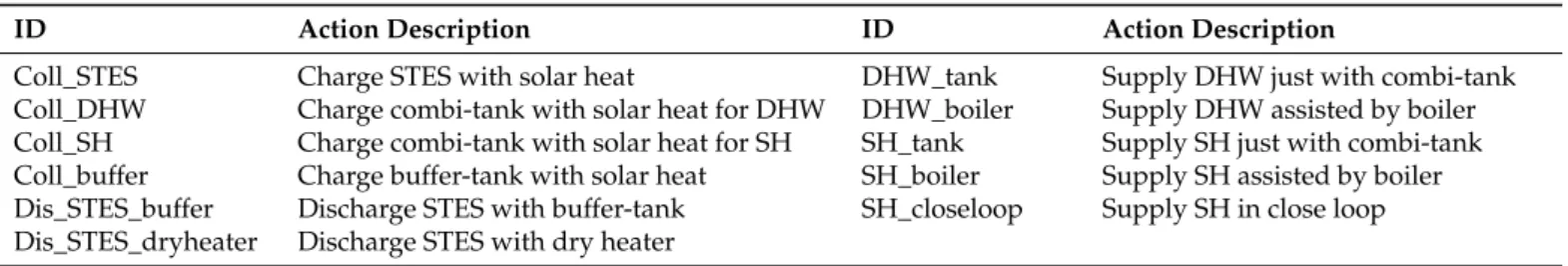
ID Action Description ID Action Description

Coll_STES Charge STES with solar heat DHW_tank Supply DHW just with combi-tank

Coll_DHW Charge combi-tank with solar heat for DHW DHW_boiler Supply DHW assisted by boiler Coll_SH Charge combi-tank with solar heat for SH SH_tank Supply SH just with combi-tank Coll_buffer Charge buffer-tank with solar heat SH_boiler Supply SH assisted by boiler Dis_STES_buffer Discharge STES with buffer-tank SH_closeloop Supply SH in close loop Dis_STES_dryheater Discharge STES with dry heater

The system under study, which is complex with a large number of operational modes and highly dependent on the weather conditions, required a control optimization to be competitive versus fossil-fuel technologies, which present an easier operation.

Section2.1explained that in summer, the sorption modules were charged at high enthalpy solar energy (i.e., >80^◦C). Solar heat at lower enthalpy was used to charge the stratified water tank. The same occurred in winter: at relatively high solar irradiation, the system charged the stratified water tank. At low enthalpy solar energy, the low temperature heat storage was charged at around 20^◦C. The optimal threshold of solar irradiation at which the operational costs of the system are minimized must be obtained through control optimization. The control threshold to be optimized, which defined the system operation, are:

1. Minimum solar irradiation in summer to charge the sorption storage tank (G_MIN,STES).

2. Minimum solar irradiation in summer to charge the stratified water tank (GMIN,COMBI,S).

3. Minimum solar irradiation in winter to charge the stratified water tank (GMIN,COMBI,W).

4. Minimum solar irradiation in winter to charge the low temperature heat source, either PCM tank or buffer water tank (GMIN,LTHS).

The control thresholds were optimized with the Hyperopt library [40] of Python. The optimization library was coupled to the RBC policy. In this way, the optimizer provided four different control thresholds to the RBC policy at every iteration. Each iteration consisted in an annual system simulation. Based on those thresholds and the RBC policy, an operational mode was selected, which in turn was given to the system simulation. At the end of the system simulation, the value of the objective function for that iteration was stored.

The optimization loop kept running until the optimizer achieved the optimum objective function. The objective function (see Equation (4)) consisted of minimizing the total annual operational costs. This total annual operational cost consisted of the gas and electrical consumption of the system as well as a cost penalty. The penalty was paid each time the SH demand was not supplied. Thus, the control will tend to maintain the middle part of

Energies2022,15, 5604 10 of 23

the stratified water tank as hot as possible to supply SH demand during the periods in which DHW and SH demand are required simultaneously.

Annual operational cost=

∑

hPF Cgas

E_nosup,DHW+E_nosup,SH

+CgasE_b+C_elE_eli (4) To calculate the objective function at each annual simulation, the following economic parameters were considered: a penalty factor (PF) of unity, a unitary cost for natural gas (Cgas) of 61.5€/MWh, and a unitary cost for electricity (C_el) of 298€/MWh (with taxes) [41] was considered. Furthermore, to calculate the electrical consumption of the dry heater, a ratio of 0.085 [39] between the thermal power rejected from the dry heater and fan electrical power consumption was considered. Eb and Eel represented the gas (at the boiler) and electrical consumption, respectively. Enosup represented the thermal demand that could not be supplied.

2.4. Case Studies

2.4.1. Building Description

The building design (see Figure7) and construction materials were obtained from the Tab- ula/Episcope database [42] using the reference building DE.N.SFH.12.Gen reported in a technical report of the SWS-heating European project [43]. The thermal transmittance of the main construction materials is shown in Table4. The same building design and construction materials were used for all the studied locations. The building model was implemented into OpenStudio Software [44]. The building had two heated thermal zones of 67 m²each and a non-heated thermal zone (attic). Using the weather data as input and using a simulation time-step of one hour, the space heating demand of the building for the different climatic files was simulated through EnergyPlus [45]. Each heated thermal zone was divided into living and sleeping areas. The temperature set-points for each thermal zone along the day are presented in Table5(obtained from a technical report of the SWS-heating European project [46]). It is important to highlight that the SH temperature set points correspond to a nearly zero-energy building [43], being part of the European Union’s goal to move towards zero-emission new buildings by 2030 [47].

Table 4.Thermal transmittance of the construction materials.

Element External Wall Floor Roof Internal Wall Ceiling

U [W/m²K] 0.11 0.12 0.05 1.7 2.9

Table 5.Heating set point schedule.

Description Heating Schedule Set Point [^◦C]

Living area weekday From 8:00 to 10:00/From 16:00 to 00:00 19 From 00:00 to 8:00/From 10:00 to 16:00 16 Living area weekend From 10:00 to 11:00/From 20:00 to 01:00 19 From 01:00 to 10:00/From 11:00 to 20:00 16 Sleeping area weekday From 21:00 to 8:00/From 17:00 to 19:00 19 From 8:00 to 17:00/From 19:00 to 21:00 16

Sleeping area weekend From 23:00 to 10:00 19

From 10:00 to 23:00 16

A DHW consumption of 90 l/day [46] with a temperature lift of 50^◦K (from 10 to 60^◦C) was con- sidered in the simulations. Both the SH and the DHW demand were interpolated to 15 min set-points.

Energies2022,15, 5604 11 of 23

Energies 2022, 15, x FOR PEER REVIEW 11 of 23

Figure 7. Sketch of the simulated building.

A DHW consumption of 90 l/day [46] with a temperature lift of 50 °K (from 10 to 60

°C) was considered in the simulations. Both the SH and the DHW demand were interpo- lated to 15 min set-points.

2.4.2. Studied Climates

The thermal performance of a sorption system is highly affected by the climatic con- ditions, which impact the ambient thermal losses and the availability of the environmental source or sink and of the solar resource. In this study, three different representative cities of central and northern Europe were studied. Paris, Munich, and Stockholm, correspond- ing to Atlantic, Continental, and Boreal biogeographical regions, respectively, according to the European Environment Agency [48]. According the Köppen climate classification, Paris corresponds to an Oceanic climate (Cfb) and Munich and Stockholm to a Humid Continental Mild Summer (Dfb). Table 6 shows the climatic properties and Table 7 the GPS coordinates and the collector’s inclination for each location. To graphically locate the three representative cities, Figure 8 places their position in a map.

Table 6. Location and climatic properties of the studied locations.

City Climate [19] Annual T^amb,avg [°C]

Winter T^amb,avg [°C]

Summer T^amb,avg [°C]

Total Annual Titled E^G [kWh/m²]

Total Summer Titled E^G [kWh/m²]

Total Winter Titled E^G [kWh/m²]

Paris Atlantic 12.5 7.8 17.2 1069 760 309

Munich Continental 9.4 3.2 15.5 1162 762 400

Stockholm Boreal 7.8 1.5 14.1 964 728 236

Table 7. GPS coordinates and inclination of solar collectors.

City Latitude [°] Longitude [°] Collector Inclination [°]

Paris 48.817 2.33 35

Munich 48.133 11.7 35

Stockholm 59.35 17.95 45

Figure 7.Sketch of the simulated building.

2.4.2. Studied Climates

The thermal performance of a sorption system is highly affected by the climatic conditions, which impact the ambient thermal losses and the availability of the environmental source or sink and of the solar resource. In this study, three different representative cities of central and northern Europe were studied. Paris, Munich, and Stockholm, corresponding to Atlantic, Continental, and Boreal biogeographical regions, respectively, according to the European Environment Agency [48].

According the Köppen climate classification, Paris corresponds to an Oceanic climate (Cfb) and Munich and Stockholm to a Humid Continental Mild Summer (Dfb). Table6shows the climatic properties and Table7the GPS coordinates and the collector’s inclination for each location. To graphically locate the three representative cities, Figure8places their position in a map.

Table 6.Location and climatic properties of the studied locations.

City Climate [19] Annual T_amb,avg[^◦C]

Winter T_amb,avg[^◦C]

Summer T_amb,avg[^◦C]

Total Annual Titled E_G [kWh/m²]

Total Summer Titled E_G [kWh/m²]

Total Winter Titled E_G [kWh/m²]

Paris Atlantic 12.5 7.8 17.2 1069 760 309

Munich Continental 9.4 3.2 15.5 1162 762 400

Stockholm Boreal 7.8 1.5 14.1 964 728 236

Table 7.GPS coordinates and inclination of solar collectors.

City Latitude [^◦] Longitude [^◦] Collector Inclination [^◦]

Paris 48.817 2.33 35

Munich 48.133 11.7 35

Stockholm 59.35 17.95 45

Meteorological data from Meteonorm [49] for Paris, Munich, and Stockholm were used in the simulations. The meteorological data consisted of average values of the period 1991–2010 with a time-step of 1 h. Figure9shows the solar global horizontal irradiation for the three studied locations.

All simulations were run in a computer with a 16 GB RAM and an Intel Core i-5 3.30 GHz processor.

Energies2022,15, 5604 12 of 23

Energies 2022, 15, x FOR PEER REVIEW 12 of 23

Figure 8. Location of three represented European cities.

Meteorological data from Meteonorm [49] for Paris, Munich, and Stockholm were used in the simulations. The meteorological data consisted of average values of the period 1991–2010 with a time-step of 1 h. Figure 9 shows the solar global horizontal irradiation for the three studied locations. All simulations were run in a computer with a 16 GB RAM and an Intel Core i-5 3.30 GHz processor.

Figure 9. Global horizontal irradiation for the three studied locations.

2.4.3. Key Performance Indicators

For analysis and comparison purposes with other systems, different performance in- dicators were defined. The thermal performance of the whole solar energy system was evaluated through the solar fraction (SF), presented in Equation (5). The solar fraction measures which percentage of the total thermal demand (D

+ D

) was covered by solar

Paris

Munich

Stockholm G H I [ W /m

] G H I [ W /m

] G H I [ W /m

]

Figure 8.Location of three represented European cities.

Energies 2022, 15, x FOR PEER REVIEW 12 of 23

Figure 8. Location of three represented European cities.

Meteorological data from Meteonorm [49] for Paris, Munich, and Stockholm were used in the simulations. The meteorological data consisted of average values of the period 1991–2010 with a time-step of 1 h. Figure 9 shows the solar global horizontal irradiation for the three studied locations. All simulations were run in a computer with a 16 GB RAM and an Intel Core i-5 3.30 GHz processor.

Figure 9. Global horizontal irradiation for the three studied locations.

2.4.3. Key Performance Indicators

For analysis and comparison purposes with other systems, different performance in- dicators were defined. The thermal performance of the whole solar energy system was evaluated through the solar fraction (SF), presented in Equation (5). The solar fraction measures which percentage of the total thermal demand (D

) was covered by solar

Paris

Munich

Stockholm GHI [W/m2]GHI [W/m2]GHI [W/m2]

Figure 9.Global horizontal irradiation for the three studied locations.

2.4.3. Key Performance Indicators

For analysis and comparison purposes with other systems, different performance indicators were defined. The thermal performance of the whole solar energy system was evaluated through the solar fraction (SF), presented in Equation (5). The solar fraction measures which percentage of the total thermal demand (D_DHW+ D_SH) was covered by solar energy, and not by fossil fuels (natural gas in this case).E_brepresents in Equation (5) the part of total thermal demand supplied by the gas boiler.

SF= (D_DHW+D_SH)−E_b

D_DHW+D_SH (5)

Energies2022,15, 5604 13 of 23

The thermal performance of a sorption storage system was analysed through the coefficient of performance (COP) and the energy density (e_d), whose numerical definitions are shown in Equations (6) and (7). The COP measures the ratio between the net discharged energy (E_ad) ver- sus the total energy required during the charging phase: the sum up of sensible (E_de,sen) plus sorption (E_de) energy. The energy density indicates the net discharged energy versus the volume of the sorbent material.

COP= ^Ead

E_de,sen+E_de (6)

e_d= ^Ead

V_sorb (7)

The COP summarizes in a single parameter the performance of the sorption storage. Neverthe- less, it depends on the charging (η_ch) and discharging efficiency (η_dis) of the sorption TES. The higher the charging and discharging efficiency, the higher the COP. The charging and discharging efficiency are calculated using the equations:

ηch= ^Ede

E_de,sen+E_de (8)

ηdis= ^Ead

E_ad,sen+E_ad (9)

The COP and the energy density have been used by many authors to evaluate the performance of sorption storage systems [10,50,51]. Nevertheless, Fumey et al. [52] reported that performance parameters such as volumetric energy density and volumetric power density are not adequate for comparison due to the highly varying conditions. Those authors proposed a new concept, called temperature effectiveness (TE), which consisted of analysing the ratio of resulting gross temperature lift in sorption (GTL_ad), compared to the required temperature lift in desorption (GTL_de). TheGTL_ad depends on the sorption temperature during discharge (T_ad,avg) and the evaporator temperature (T_e,avg). On the other side, theGTL_de depends on the desorption temperature (T_de,avg) and the condensing temperature (Tc,avg) The temperature effectiveness of the STES system under study was calculated using the following equations [52]:

TEavg= ^GTLad

GTL_de (10)

GTL_ad=T_ad,avg−Te,avg (11)

GTL_de=T_de,avg−Tc,avg (12)

With regard to the system analysis from an environmental approach, the CO₂emissions saved by the solar system at each location were analysed. The CO2emissions were calculated by multiplying the annual thermal demand supplied by the solar seasonal system, divided by the boiler efficiency (i.e., 0.9), by the equivalent CO₂emissions (0.18 kg/kWh) [53].

3. Results and Discussion 3.1. Overall System Results

The three studied scenarios were analysed for one year under optimal control policy. Solar irradiation, ambient temperature, and thermal demand of each location have large impacts on the selected system operational mode. The optimal control must search, among other aspects, for the best trade-off between maximum solar heat stored in the sorption system in summer, discharged energy by the sorption system given the winter weather conditions, and solar heat that can be directly supplied to the stratified water tank.

The sorption system temperature decreases due to the thermal losses to the ambient, especially in summer. The longer the intervals between two consecutive charges or discharges, the higher the sensible heat required to reach the regeneration or sorption temperature of the sorbent material, which causes a decrease in the efficiency. From an overall system perspective, during some periods, it may be more efficient and cost-effective to charge the stratified water tank with solar heat than the sorption modules or the low temperature heat source. Hence, the optimal irradiation control thresholds were set to operate the sorption modules only when it was more cost-effective, despite the fact that its full capacity was not exploited.

The optimal control thresholds of the RBC strategy are presented in Table8. Stockholm was the location with the lowest solar irradiation in winter (see Table6), but with the highest space heating demand. Especially in this climate, solar heat stored during summer in the sorption system will

Energies2022,15, 5604 14 of 23

be necessary in winter for SH application. Thus, the optimal economic scenario was obtained for a threshold-1 of 421 W/m²(see Table8), a value considerably lower compared to Paris and Munich.

This threshold made it possible that in summer, when the solar irradiation was above this value, the sorption system was charged, reaching a maximum state of charge (SoC) of 76% in spite of the lower solar availability. The maximum SoC of the sorption system in Munich, which presented the higher annual total solar irradiation and a thermal demand of 9.88 MWh, was 84 %. The overall system main results for the three studied cities are presented in Tables9and10.

Table 8.Optimal control thresholds.

City G_MIN,STES GMIN,COMBI,S GMIN,COMBI,W G_MIN,LTHS

Paris [W/m²] 475 172 115 81

Munich [W/m²] 464 126 120 80

Stockholm

[W/m²] 421 88 133 82

Table 9.Overall system KPIs for the studied locations.

City Annual Cost [€] SF [%] CO₂Emissions Savings [kg] Maximum SoC [%]

Paris 274.9 44.5 576 93.1

Munich 444.8 40.8 808 84.0

Stockholm 706.2 27.0 697 78.2

Table 10.Supplied energy demand and generated solar energy for each location.

City Total Thermal

Demand

Thermal Demand Supplied by

System

Thermal Demand Supplied by

Boiler

Energy Generated by

Solar Field

Paris [MWh] 6.46 2.88 3.58 6.43

Munich

[MWh] 9.88 4.04 5.84 7.17

Stockholm

[MWh] 12.91 3.48 9.42 5.63

The system obtained solar fractions of 44.5, 40.8, and 27.0% in Paris, Munich, and Stockholm, respectively. The highest solar fraction was reached for Paris due to its higher ratio between total annual solar irradiation (1069 kWh/m²) and thermal demand (6.46 MWh). The second highest solar fraction was obtained for Munich, which presented higher total annual solar irradiation compared to Paris (8%), but also higher annual thermal demand (9.88 MWh). Stockholm obtained the lowest solar fraction due to its lower solar energy availability (963.8 kW/m²) and its much higher thermal demand compared to Paris and Munich (2 and 1.3 times more, respectively).

In absolute terms, the solar seasonal system operated under Munich weather conditions sup- plied the maximum amount of energy to the demand: 4.04 MWh (without fossil fuel support) and therefore saved the maximum amount of CO₂emissions: 808 kg. The best solar conversion rate (energy generated by the solar field vs. thermal demand supplied by the solar seasonal system) was reached by Stockholm. Its higher space heating in intermediate seasons made it possible to profit better from solar energy.

3.2. Thermal Performance of Sorption Storage

Table11presents the KPIs of the sorption storage system for the three studied climates: Paris, Munich, and Stockholm. In the proposed system, the discharge of the sorption modules depended on a low temperature heat source charged by low enthalpy solar heat (see Table8for solar irradiation thresholds). Hence, the discharge of the sorption system during winter depended on the solar irradiation. To maximize the system efficiency and minimize the operational costs, the optimal control should choose the scenario in which all the energy stored in the sorption system during summer can be discharged by the end of the winter. The system located in Paris reached the highest charging rate (SoC of 91%). Nevertheless, Paris presented a total winter solar irradiation of 309 kWh/m²), which could limit the discharging of the sorption system. Nonetheless, thanks to

Energies2022,15, 5604 15 of 23

the high ambient temperatures during winter (TAMB,AVG,W= 7.8^◦C) and the use of a dry heater that profits from ambient heat to assist the evaporator, the sorption storage could discharge 91% of its total capacity. In Paris, the dry heater prolonged the discharging of the sorption storage during 112 h per year. The integration of a dry heater to profit ambient heat was explored also under Munich weather conditions. Nevertheless, the dry heater was only used for 9.5 h due to the low ambient temperatures during winter. The few hours of dry-heater operation did not justify its use during winter under climates as Munich or more severe ones. For this reason, in this study the implementation of a dry heater was just considered for Paris. Nonetheless, Munich and Stockholm presented similar sorption storage discharging efficiency (around 69.5%) thanks to the optimization of the system operation.

Table 11.KPIs of the sorption storage system.

City Use of STES [%] COP TE ed[kWh/m³] ηCH, STES[%] ηDIS, STES[%]

Paris 91 0.284 0.384 106.2 42.4 69.0

Munich 82 0.277 0.357 96.7 40.8 70.3

Stockholm 76 0.311 0.320 88.5 46.7 68.8

With respect to energy density, Paris reached the hi