STATUS OF NEUTRINO OSCILLATION EXPERIMENTS

(1)

STATUS OF NEUTRINO OSCILLATION EXPERIMENTS

H. A. Tanaka (SLAC, Stanford University)

(2)

QUICK OVERVIEW:

• Thank you to the INVISIBLES organizers for this opportunity to participate in this workshop!

• Here, I will focus mainly on “long baseline accelerator-based” neutrino oscillation experiments

• Quickly review relevant neutrino oscillation phenomenology

• Others will discuss “short baseline” experiments

(3)

NEUTRINO OSCILLATIONS

• Neutrino come in three “flavor” eigenstates ( ν e , ν µ , ν τ )

• Likewise, neutrinos come in three mass eigenstates ( ν 1 , ν 2 , ν 3 )

• The mass and flavor eigenstates “mix” (summarized in unitary matrix U)

• Neutrinos are produced in flavor eigenstates by weak interaction

• Mass eigenstates evolve differently in proper time (L/E).

• New flavor components appear → “neutrino oscillations”

!3

e - , µ - , τ - W

ν e, µ, τ

| ⌫

↵

i = X

i

U

_↵i^⇤

| ⌫

i

• Amplitudes from mixing matrix U

• Wavelength in L/E ν by mass 2 splittings.

2 13. Neutrino mixing

Here, E i and p i are respectively the energy and momentum of ν i in the laboratory frame. In practice, our neutrino will be extremely relativistic, so we will be interested in evaluating the phase factor of Eq. (13.4) with t ≈ L, where it becomes exp[ − i(E i − p i )L].

Imagine now that our ν α has been produced with a definite momentum p, so that all of its mass-eigenstate components have this common momentum. Then the ν i component has E i = !

p 2 + m 2 i ≈ p + m 2 i /2p, assuming that all neutrino masses m i are small compared to the neutrino momentum. The phase factor of Eq. (13.4) is then approximately

e − i(m 2 i /2 p)L . (13.5)

From this expression and Eq. (13.1), it follows that after a neutrino born as a ν α has propagated a distance L, its state vector has become

| ν α (L) ⟩ ≈ "

i

U αi ∗ e − i(m 2 i /2 E)L | ν i ⟩ . (13.6)

Here, E ≃ p is the average energy of the various mass eigenstate components of the neutrino. Using the unitarity of U to invert Eq. (13.1), and inserting the result in Eq. (13.6), we find that

| ν α (L) ⟩ ≈ "

β

# "

i

U αi ∗ e − i(m 2 i /2 E)L U βi

$

| ν β ⟩ . (13.7)

We see that our ν α , in traveling the distance L, has turned into a superposition of all the flavors. The probability that it has flavor β, P (ν α → ν β ), is obviously |⟨ ν β | ν α (L) ⟩| 2 . From Eq. (13.7) and the unitarity of U , we easily find that

P (ν α → ν β ) = δ αβ

− 4 "

i>j

ℜ (U αi ∗ U βi U αj U βj ∗ ) sin 2 [1.27 ∆m 2 ij (L/E)]

+2 "

i>j

ℑ (U αi ∗ U βi U αj U βj ∗ ) sin[2.54 ∆m 2 ij (L/E)] . (13.8)

Here, ∆m 2 ij ≡ m 2 i − m 2 j is in eV 2 , L is in km, and E is in GeV. We have used the fact that when the previously omitted factors of ! and c are included,

∆m 2 ij (L/4E) ≃ 1.27 ∆m 2 ij (eV 2 ) L(km)

E(GeV) . (13.9)

The quantum mechanics of neutrino oscillation leading to the result Eq. (13.8) is somewhat subtle. To do justice to the physics requires a more refined treatment [3] than the one we have given. Sophisticated treatments continue to yield new insights [4].

July 14, 2006 10:37

Δm 2ij (eV 2 ) L (km) E (GeV)

P( ν e →ν e ) vs. L/E ν

(4)

THREE FLAVORS

• Observation of neutrino oscillations in atmospheric neutrinos:

• Mass 2 splitting of 2.5x10 -3 eV 2 (Δm 2atm )

• First maximum at 500 km/GeV

• Solar/reactor experiments:

• Another mass 2 splitting is ~7.8x10 -5 eV 2 (Δm 2sol )

0

@ ⌫ e

⌫ µ

⌫ ⌧

1 A =

0

@ U e1 ⇤ U e2 ⇤ U e3 ⇤ U µ1 ⇤ U µ2 ⇤ U µ3 ⇤ U ⌧1 ⇤ U ⌧2 ⇤ U ⌧3 ⇤

1 A

0

@ ⌫ 1

⌫ 2

⌫ 3

1 A

13. Neutrino mixing 13

ν 1 ν 2 ν 3

U = ν e ν µ ν τ

⎡

⎣ c 12 c 13 s 12 c 13 s 13 e −iδ

− s 12 c 23 − c 12 s 23 s 13 e iδ c 12 c 23 − s 12 s 23 s 13 e iδ s 23 c 13 s 12 s 23 − c 12 c 23 s 13 e iδ − c 12 s 23 − s 12 c 23 s 13 e iδ c 23 c 13

⎤

⎦

× diag(e iα

¹

/2 , e i α

²

/2 , 1) . (13.31) Here, ν 1 and ν 2 are the members of the solar pair, with m 2 > m 1 , and ν 3 is the isolated neutrino, which may be heavier or lighter than the solar pair. Inside the matrix, c ij ≡ cos θ ij and s ij ≡ sin θ ij , where the three θ ij ’s are mixing angles. The quantities δ, α 1 , and α 2 are CP -violating phases. The phases α 1 and α 2 , known as Majorana phases, have physical consequences only if neutrinos are Majorana particles, identical to their antiparticles. Then these phases influence neutrinoless double beta decay [see Sec. IV] and other processes [32]. However, as we see from Eq. (13.8), α 1 and α 2 do not aﬀect neutrino oscillation, regardless of whether neutrinos are Majorana particles.

Apart from the phases α 1 , α 2 , which have no quark analogues, the parametrization of the leptonic mixing matrix in Eq. (13.31) is identical to that [33] advocated for the quark mixing matrix by Gilman, Kleinknecht, and Renk in their article in this Review.

From bounds on the short-distance oscillation of reactor ν e [8] and other data, at 2 σ, | U e3 | 2 < ∼ 0.032 [34]. (Thus, the ν e fraction of ν 3 would have been too small to see in Fig. 13.3; this is the reason it was neglected.) From Eq. (13.31), we see that the bound on | U e3 | 2 implies that s 2 13 < ∼ 0.032. From Eq. (13.31), we also see that the CP-violating phase δ, which is the sole phase in the U matrix that can produce CP violation in neutrino oscillation, enters U only in combination with s 13 . Thus, the size of CP violation in oscillation will depend on s 13 .

Given that s 13 is small, Eqs. (13.31), (13.14), and (13.16) imply that the atmospheric mixing angle θ atm extracted from ν µ disappearance measurements is approximately θ 23 , while Eqs. (13.31) and (13.17) (with ν α = ν e and θ = θ ⊙ ) imply that θ ⊙ ≃ θ 12 .

If the LSND oscillation is confirmed, then, as already noted, there must be at least four mass eigenstates. It is found that if there are exactly four, a statistically satisfactory fit to all the neutrino data is not possible. However, if there are at least four neutrino mass eigenstates, there is no strong reason to believe that there are exactly four. The presence of more states may improve the quality of the fit. For example, it has been found that a “3+2” spectrum fits all the short-baseline data significantly better than a 3+1 spectrum [35].

IV. The neutrino-anti-neutrino relation: Unlike quarks and charged leptons, neutrinos may be their own antiparticles. Whether they are depends on the nature of the physics that gives them mass.

In the Standard Model (SM), neutrinos are assumed to be massless. Now that we know they do have masses, it is straightforward to extend the SM to accommodate these masses in the same way that this model accommodates quark and charged lepton masses.

When a neutrino ν is assumed to be massless, the SM does not contain the chirally

s ij = sin θ ij c ij = cos θ ij

• Three rotation angles ( θ 12 , θ 13 , θ 23 )

• One complex phase δ CP

• additional phases possible if neutrinos are “Majorana”

• changes sign for antineutrino oscillations (“CP odd”)

(5)

THE MATTER DOMINATED UNIERSE

!5

• Extremely small?

• Extremely large?

• Known sources of CPV (quark mixing) cannot produce this asymmetry

1

MATTER ANTI-MATTER

MATTER

figure courtesy of H.

Murayama

Challenge to Particle Physics

HOW DID THIS HAPPEN?

B

N ⇠ O (10 10 )

Further exploration and elucidation of possible CPV sources is critical

S A K H A R O V C O N D I T I O N S :

• B A RY O N N U M B E R ( B ) V I O L AT I O N

• V I O L AT I O N O F C , C P S Y M M E T RY ( C P V )

• D E PA R T U R E F R O M T H E R M A L E Q U I L I B R I U M

(6)

ACCELERATOR-BASED BEAMS

(7)

NEUTRINO BEAMS IN A NUTSHELL

• To first order, accelerator-based neutrino beams operate on the same basic principles

!7

1

2 3 4

1. High energy protons impinge on a target

• pions are produced

2. Electromagnets focus pions into a decay region

• one sign is focussed, the other defocussed 3. The pions decay in a decay pipe

• muon (anti)neutrinos are produced

4. Beam absorber stops all other remaining particles

• some muons penetrate and can be monitored.

• neutrinos go on to the experiment

• Each step represents an enormous technical challenge

• Primary proton beams approaching 1 MW in power

• Hundreds of kA of current to focus the beam

Currency: “protons-on-target”

Non-trivial exchange rate when

comparing different beams

(8)

LONG BASELINE EXPERIMENTS

Accelerator-based beams are typically E ν ~ few GeV

• “on-axis” beams provide the highest rate, width of spectrum

• “off-axis” beams tuned to maximize the oscillation probability, reduce background

Maximize oscillations for Δm 2atm → 500 km/GeV

Large O(10%) uncertainties in flux, ν interaction modeling

P (⌫ µ ! ⌫ µ ) ⇠ 1 (cos 4 ✓ 13 sin 2 2✓ 23 + sin 2 2✓ 13 sin 2 ✓ 23 ) sin 2 (1.27 m 2 31 L/E ) !8

<latexit sha1_base64="XJShGjG6REG3U4YWOHuZ2hC1kf4=">AAACeXicbZHLbhMxFIY9w60Nl6ZlCQtDVDShahhPKpVlxUViwSJIpK2USUYe56SxantG9hmkaJR34NnY8SLdsMFJB1EajmTp1/f/R7bPyUslHcbxzyC8c/fe/Qdb262Hjx4/2Wnv7p26orIChqJQhT3PuQMlDQxRooLz0gLXuYKz/PL9yj/7BtbJwnzFRQljzS+MnEnB0aOs/X0QpabKUl3RFAva6C5NndSU0UMapaJwkyPvzgF5VrP+cmWaSUKTPyzx7GCD/k3eyHUbFLFeckzTD6CQUz1JsrrPlp/ffOxm7U7ci9dFNwVrRIc0NcjaP9JpISoNBoXizo1YXOK45halULBspZWDkotLfgEjLw3X4Mb1enJLuu/JlM4K649BuqY3O2qunVvo3Cc1x7m77a3g/7xRhbO341qaskIw4vqiWaWon/FqDXQqLQhUCy+4sNK/lYo5t1ygX1bLD4Hd/vKmOE16zOsvR52Td804tsgz8pJEhJFjckI+kQEZEkGugufBfvAq+BW+CKPw9XU0DJqep+SfCvu/AXgWumU=</latexit><latexit sha1_base64="XJShGjG6REG3U4YWOHuZ2hC1kf4=">AAACeXicbZHLbhMxFIY9w60Nl6ZlCQtDVDShahhPKpVlxUViwSJIpK2USUYe56SxantG9hmkaJR34NnY8SLdsMFJB1EajmTp1/f/R7bPyUslHcbxzyC8c/fe/Qdb262Hjx4/2Wnv7p26orIChqJQhT3PuQMlDQxRooLz0gLXuYKz/PL9yj/7BtbJwnzFRQljzS+MnEnB0aOs/X0QpabKUl3RFAva6C5NndSU0UMapaJwkyPvzgF5VrP+cmWaSUKTPyzx7GCD/k3eyHUbFLFeckzTD6CQUz1JsrrPlp/ffOxm7U7ci9dFNwVrRIc0NcjaP9JpISoNBoXizo1YXOK45halULBspZWDkotLfgEjLw3X4Mb1enJLuu/JlM4K649BuqY3O2qunVvo3Cc1x7m77a3g/7xRhbO341qaskIw4vqiWaWon/FqDXQqLQhUCy+4sNK/lYo5t1ygX1bLD4Hd/vKmOE16zOsvR52Td804tsgz8pJEhJFjckI+kQEZEkGugufBfvAq+BW+CKPw9XU0DJqep+SfCvu/AXgWumU=</latexit><latexit sha1_base64="XJShGjG6REG3U4YWOHuZ2hC1kf4=">AAACeXicbZHLbhMxFIY9w60Nl6ZlCQtDVDShahhPKpVlxUViwSJIpK2USUYe56SxantG9hmkaJR34NnY8SLdsMFJB1EajmTp1/f/R7bPyUslHcbxzyC8c/fe/Qdb262Hjx4/2Wnv7p26orIChqJQhT3PuQMlDQxRooLz0gLXuYKz/PL9yj/7BtbJwnzFRQljzS+MnEnB0aOs/X0QpabKUl3RFAva6C5NndSU0UMapaJwkyPvzgF5VrP+cmWaSUKTPyzx7GCD/k3eyHUbFLFeckzTD6CQUz1JsrrPlp/ffOxm7U7ci9dFNwVrRIc0NcjaP9JpISoNBoXizo1YXOK45halULBspZWDkotLfgEjLw3X4Mb1enJLuu/JlM4K649BuqY3O2qunVvo3Cc1x7m77a3g/7xRhbO341qaskIw4vqiWaWon/FqDXQqLQhUCy+4sNK/lYo5t1ygX1bLD4Hd/vKmOE16zOsvR52Td804tsgz8pJEhJFjckI+kQEZEkGugufBfvAq+BW+CKPw9XU0DJqep+SfCvu/AXgWumU=</latexit><latexit sha1_base64="XJShGjG6REG3U4YWOHuZ2hC1kf4=">AAACeXicbZHLbhMxFIY9w60Nl6ZlCQtDVDShahhPKpVlxUViwSJIpK2USUYe56SxantG9hmkaJR34NnY8SLdsMFJB1EajmTp1/f/R7bPyUslHcbxzyC8c/fe/Qdb262Hjx4/2Wnv7p26orIChqJQhT3PuQMlDQxRooLz0gLXuYKz/PL9yj/7BtbJwnzFRQljzS+MnEnB0aOs/X0QpabKUl3RFAva6C5NndSU0UMapaJwkyPvzgF5VrP+cmWaSUKTPyzx7GCD/k3eyHUbFLFeckzTD6CQUz1JsrrPlp/ffOxm7U7ci9dFNwVrRIc0NcjaP9JpISoNBoXizo1YXOK45halULBspZWDkotLfgEjLw3X4Mb1enJLuu/JlM4K649BuqY3O2qunVvo3Cc1x7m77a3g/7xRhbO341qaskIw4vqiWaWon/FqDXQqLQhUCy+4sNK/lYo5t1ygX1bLD4Hd/vKmOE16zOsvR52Td804tsgz8pJEhJFjckI+kQEZEkGugufBfvAq+BW+CKPw9XU0DJqep+SfCvu/AXgWumU=</latexit>

5

DUNE XSEC model

● DUNEInt package – heavily augmented GENIE model

● Benefit from T2K, NOvA and MINERvA experience, which spans the energy region of interest

● Theory developments expected and required, but we can build an empirical model to estimate model deficiencies

Since the beam is ν µ or ν µ , a critical measurement is the

“disappearance” of ν µ / ν µ into other flavors

• θ 13 from reactor ν e disappearance: sin 2 θ 13 =2.18±0.07x10 -3

• Primarily sensitive to sin 2 2 θ 23

(9)

ν μ → ν e OSCILLATION PROBABILITY

• θ 13 may be constrained by reactor measurements

• θ 23 (as opposed to 2 θ 23 ) dependence → “octant” matters if θ 23 ≠45°

• Joint analysis with ν µ disappearance

• CP odd phase δ CP can result in

• asymmetry of oscillation probabilities P( ν µ →ν e ) ≠ P( ν µ →ν e ), distortion of ν e / ν e

• Mass ordering sensitivity through x : ν e / ν e enhanced in normal/inverted hierarchy !9

P (⌫ µ ! ⌫ e ) ⇠ sin 2 2✓ 13 ⇥ sin 2 ✓ 23 ⇥ sin 2 (1 [(1 x) x) ] 2

↵ sin ⇥ sin 2✓ 12 sin 2✓ 13 sin 2✓ 23 ⇥ sin sin[x x ] sin[(1 (1 x) x) ] +↵ cos ⇥ sin 2✓ 12 sin 2✓ 13 sin 2✓ 23 ⇥ cos sin[x x ] sin[(1 (1 x) x) ] + O (↵ 2 )

⌘ m 2 31 L

↵ = m 2 21 4E

m 2 31 ⇠ 1

30 x = ±

2 p

2G F N e E ⌫ m 2 31

<latexit sha1_base64="tjo3am/CSYW2H1rTzVxsiPKC8yI=">AAACIXicdVBNaxRBEO2JUeP6tdFjLkUWwdPSMya6OQhBTfQUIrhJYGcdenprkibdPZPuGnEZ5q948a948RCR3MQ/k97NCir6oODxXhVV9fJKK0+c/4iWri1fv3Fz5Vbn9p279+53Vx8c+LJ2Eoey1KU7yoVHrSwOSZHGo8qhMLnGw/z05cw//IDOq9K+o2mFYyOOrSqUFBSkrDv4CM8hrQykhROySVJ/5qhJWnid7cJehrCTpbZuoUlfoSYB5n2SNU/its26Pd7f5PHW0xh4n88RSLLJtwYc4oXSYwvsZ92LdFLK2qAlqYX3o5hXNG6EIyU1tp209lgJeSqOcRSoFQb9uJl/2MKjoEygKF0oSzBXf59ohPF+avLQaQSd+L+9mfgvb1RTMRg3ylY1oZVXi4paA5UwiwsmyqEkPQ1ESKfCrSBPRIiKQqidEMKvT+H/5CDpx4G/3ehtv1jEscLW2Dp7zGL2jG2zN2yfDZlkn9gXds6+RZ+jr9H36OKqdSlazDxkfyD6eQkTk6JA</latexit><latexit sha1_base64="tjo3am/CSYW2H1rTzVxsiPKC8yI=">AAACIXicdVBNaxRBEO2JUeP6tdFjLkUWwdPSMya6OQhBTfQUIrhJYGcdenprkibdPZPuGnEZ5q948a948RCR3MQ/k97NCir6oODxXhVV9fJKK0+c/4iWri1fv3Fz5Vbn9p279+53Vx8c+LJ2Eoey1KU7yoVHrSwOSZHGo8qhMLnGw/z05cw//IDOq9K+o2mFYyOOrSqUFBSkrDv4CM8hrQykhROySVJ/5qhJWnid7cJehrCTpbZuoUlfoSYB5n2SNU/its26Pd7f5PHW0xh4n88RSLLJtwYc4oXSYwvsZ92LdFLK2qAlqYX3o5hXNG6EIyU1tp209lgJeSqOcRSoFQb9uJl/2MKjoEygKF0oSzBXf59ohPF+avLQaQSd+L+9mfgvb1RTMRg3ylY1oZVXi4paA5UwiwsmyqEkPQ1ESKfCrSBPRIiKQqidEMKvT+H/5CDpx4G/3ehtv1jEscLW2Dp7zGL2jG2zN2yfDZlkn9gXds6+RZ+jr9H36OKqdSlazDxkfyD6eQkTk6JA</latexit><latexit sha1_base64="tjo3am/CSYW2H1rTzVxsiPKC8yI=">AAACIXicdVBNaxRBEO2JUeP6tdFjLkUWwdPSMya6OQhBTfQUIrhJYGcdenprkibdPZPuGnEZ5q948a948RCR3MQ/k97NCir6oODxXhVV9fJKK0+c/4iWri1fv3Fz5Vbn9p279+53Vx8c+LJ2Eoey1KU7yoVHrSwOSZHGo8qhMLnGw/z05cw//IDOq9K+o2mFYyOOrSqUFBSkrDv4CM8hrQykhROySVJ/5qhJWnid7cJehrCTpbZuoUlfoSYB5n2SNU/its26Pd7f5PHW0xh4n88RSLLJtwYc4oXSYwvsZ92LdFLK2qAlqYX3o5hXNG6EIyU1tp209lgJeSqOcRSoFQb9uJl/2MKjoEygKF0oSzBXf59ohPF+avLQaQSd+L+9mfgvb1RTMRg3ylY1oZVXi4paA5UwiwsmyqEkPQ1ESKfCrSBPRIiKQqidEMKvT+H/5CDpx4G/3ehtv1jEscLW2Dp7zGL2jG2zN2yfDZlkn9gXds6+RZ+jr9H36OKqdSlazDxkfyD6eQkTk6JA</latexit><latexit sha1_base64="tjo3am/CSYW2H1rTzVxsiPKC8yI=">AAACIXicdVBNaxRBEO2JUeP6tdFjLkUWwdPSMya6OQhBTfQUIrhJYGcdenprkibdPZPuGnEZ5q948a948RCR3MQ/k97NCir6oODxXhVV9fJKK0+c/4iWri1fv3Fz5Vbn9p279+53Vx8c+LJ2Eoey1KU7yoVHrSwOSZHGo8qhMLnGw/z05cw//IDOq9K+o2mFYyOOrSqUFBSkrDv4CM8hrQykhROySVJ/5qhJWnid7cJehrCTpbZuoUlfoSYB5n2SNU/its26Pd7f5PHW0xh4n88RSLLJtwYc4oXSYwvsZ92LdFLK2qAlqYX3o5hXNG6EIyU1tp209lgJeSqOcRSoFQb9uJl/2MKjoEygKF0oSzBXf59ohPF+avLQaQSd+L+9mfgvb1RTMRg3ylY1oZVXi4paA5UwiwsmyqEkPQ1ESKfCrSBPRIiKQqidEMKvT+H/5CDpx4G/3ehtv1jEscLW2Dp7zGL2jG2zN2yfDZlkn9gXds6+RZ+jr9H36OKqdSlazDxkfyD6eQkTk6JA</latexit>

(10)

QUICK SUMMARY

• increase sin 2 θ 23 , sin 2 2 θ 13

• enhance both ν µ →ν e and ν µ →ν e

• CP violating parameter δ CP

• δ CP =0,π: no CP violation: vacuum oscillation probabilities equal

• δ CP ~-π/2: enhance ν µ →ν e , suppress ν µ →ν e

• δ CP ~+π/2: suppress ν µ →ν e , enhance ν µ →ν e

Mayly Sanchez - ISU

N O VA’ S P H Y S I C S G O A L S

! 4

What is the mass hierarchy or ordering for atmospheric neutrinos?  

Is there a ν μ - ν τ symmetry (is the large mixing angle maximal; if not, what is the octant)?  

Is CP violated in the lepton sector?  

Are there other neutrinos beyond the three known active flavors?

T H E N O VA P R O G R A M S E E K S T O A N S W E R K E Y U N K N O W N S N E U T R I N O A N D A N T I N E U T R I N O D ATA A R E R E Q U I R E D

20 30 40 50 60 70 80

Total events - neutrino mode

5 10 15 20 25

Total events - antineutrino mode

_{= 0}

δCP δ_CP= π/2

= π

δCP δ_CP= 3π/2 eV2

10-3

2.55×

=−

2

m32

Δ IH

eV2

10-3

2.50×

=+

2

m32

Δ NH

=0.46 θ23

sin2

LO sin²θ₂₃=0.59

UO

=0.082 θ13 22 NOvA FD sin

) ν POT ( 1020

× 9.48

ν) POT ( 1020

6.91×

< 0

> 0

< 0 . 5

> 0 . 5 I N V E R T E D H I E R A R C H Y ( I H )

N O R M A L H I E R A R C H Y ( N H )

20 30 40 50 60 70 80

5 10 15 20 25

Total events - antineutrino mode

_{= 0}

δCP δ_CP= π/2 π

CP=

δ δ_CP= 3π/2 eV2

10-3

2.55×

=−

2

m32

Δ IH

eV2

10-3

× 2.50 +

2= m32

Δ NH

=0.46 θ23

sin2

LO sin²θ₂₃=0.59

UO

=0.082 θ13 22 NOvA FD sin

ν) POT ( 1020

9.48×

ν) POT ( 1020

6.91×

L O W E R O C TA N T ( L O )

U P P E R O C TA N T ( U O )

F I R S T N O VA A N T I N E U T R I N O D ATA AT T H I S C O N F E R E N C E

• “normal” ordering:

• enhance ν µ →ν e

• suppresses ν µ →ν e

• “inverted” ordering:

• suppress ν µ →ν e

• enhance ν µ →ν e

(11)

TOKAI-TO-KAMIOKA (T2K)

Super Kamiokande

“far” detector

ND280

“near” detector

• “Long baseline” experiment

• Shoot a ~600 MeV muon (anti)neutrino beam from one side of Japan to the other

• 295 km distance from J-PARC (in Tokai) to Kamioka → 500 km/GeV

!11 Tokai

Kamioka

295 km

ν: 14.9x10 20 POT, ν : 16.4x10 20 POT

(12)

CHERENKOV RADIATION

α θ C

• Analogous to other (mechanical) systems where a disturbance exceeds the propagation velocity

• e.g. “sonic boom” from supersonic object

sin ↵ = v s

v ↵ = ⇡

2 ✓ C

courtesy findagrave.com

(13)

EVENTS AT T2K

!13 e-like (“1Re”)

μ-like (“1Rμ”)

Signal “CCQE”

“NC 1π”

+ n ⇥ + p

+ p + p + ⇥ 0

n p

“CCQE” W

p

+

0

Z Multi-ring

• At ~600 MeV, neutrino interactions tend to have low “multiplicity”

• Typically “quasi-elastic” lepton + nucleon topology

• With proton typically below Cherenkov threshold, signature is a single ring “1R” from the electron or muon

(14)

NOvA

!14

• ~2 GeV ν µ /ν µ beam produced at Fermilab

• More complex neutrino interactions (e.g. pion production)

• Sent 810 km to the NOvA detector in Minnesota

• 14 kt liquid scintillating detector

• Maintain L/E ~500 km/GeV corresponding to Δm 2 ~ 2.5 x 10 -3 eV 2

ν: 8.85x10 20 POT, ν : 6.91x10 20 POT

(15)

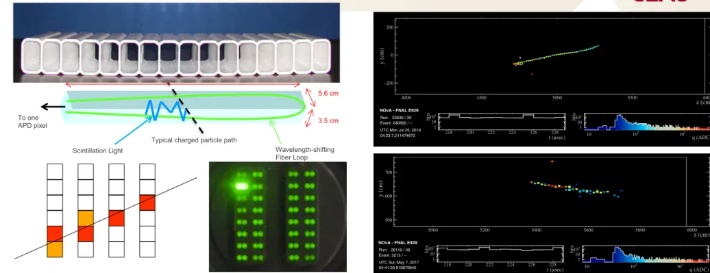
NOvA DETECTOR CONCEPT

!15 1

2 twice as long as the extrusion and looped at the “far end” of the cell (Fig. 1). Generally, the scintillation light is captured by the WLS fiber after several reflections off the cell walls.

Simulations show that scintillation light reflects about 8 times on average before entering the fiber. This is the key reason to use highly-reflective PVC surfaces. The Far Detector has a total of 344,064 PVC cells, individually equipped with optical fibers to transport scintillation light to a 32-channel avalanche photodiode (APD) that sits just over an optical connector attached to each 32 cell module.

Figure 1: Ionizing particles passing through the scintillating liquid contained within an extrusion cell produce light, which reflects off the PVC walls multiple times until being captured by a wavelength shifting fiber optic loop. Light within the fiber optic travels the length of the extrusion and is detected by an avalanche photodiode (APD). Dimensions refer to liquid volume.

Detector Structure

The extrusions form the mechanical backbone of the NOvA detectors, providing the strength necessary to maintain a very large structure filled with liquid scintillator. In order to capture the scintillation light for readout, the extrusion cell walls must have a high reflectance; significantly higher than found in commercial PVC products. We have developed a PVC-based formulation to achieve high reflectance while maintaining the necessary mechanical strength. This paper describes the techniques developed to produce more than 11 million pounds of NOvA extrusions that meet strict reflectance, strength and dimensional requirements. An extrusion profile schematic is shown in Fig. 2, and a photograph in Fig. 3a.

Figure 2: NOvA extrusion cross section with cells numbered 1 through 16 (dimensions are in millimeters).

The Near and Far Detectors consist of free-standing blocks of PVC extrusions, filled with liquid scintillator. The NOvA Far Detector is at this time potentially the largest self-supporting plastic structure ever built. Although the primary purpose of this paper is to describe PVC extrusion development, a brief description of the detector assembly process is helpful to provide context for the physical and optical requirements of PVC extrusions as detector elements.

Typical charged particle path To one

APD pixel

L = 15.5 m

3.5 cm 5.6 cm

Scintillation Light Wavelength-shifting

Fiber Loop

3

Figure 3: (a) Close-up photos of one 16-cell PVC extrusion, 15 cm long. (b) Two full-size 16-cell extrusions 15.5 m long placed side-by side form the basis for an extrusion module.

After the 16-cell PVC extrusions were produced, they were shipped to the University of Minnesota to be assembled into the basic detector element of NOvA: the extrusion module. A module consists of an instrumented pair of 16-cell extrusions, each 63.5 cm wide and 15.5 m (3.9 m) long for the Far Detector (Near Detector). To make a module, first a pair of extrusions was bonded side-to-side, resulting in a 32-cell object 1.27 m wide as shown in Fig 3b. This was done to maximize efficient use of readout electronics, which is based on 32 channels. Y-11 wavelength shifting fiber (0.7 mm diameter) [REF 3] was inserted down the entire length of each cell and looped around a fixture at the far end, for a total length of approximately 33 meters per cell, depending on the routing distance in the manifold to the optical connector. At the near end, both ends of the fiber were routed inside a manifold to terminate at an optical connector. Both ends of the extrusions were sealed with the aid of custom-made plastic gaskets and adhesive. The near end of a module was sealed with an injection-molded cover that enveloped the fiber manifold and exposed the optical connector. The far end of the module was sealed with a flat PVC plate that was designed to bear a structural load.

The third and final step of the detector assembly process was performed at the experimental sites: Ash River Minnesota (Far Detector) and Fermilab (Near Detector). Both locations required excavation and construction of specialized laboratory detector halls, oriented along the direction of the neutrino beam (approximately a north-south direction). Extrusion modules were shipped from the University of Minnesota to these sites, where they were assembled into detector blocks and placed in position to form the Far and Near Detectors. Because the Far Detector is significantly larger than the Near Detector, PVC extrusions were designed and built to meet the extraordinary size, stress and reflectance criteria necessitated by its requirements. We therefore limit the detector assembly procedure discussion to the Far Detector.

The Far Detector assembly process for each Far Detector Block (FDB) is described in brief.

First, twelve extrusion modules were put down next to each other on an assembly platform table.

Since each module is 15.5 m long and 1.27 m wide, the twelve modules form a square 15.5 m on a side, with the extruded cells oriented in a north-south direction. A second layer of twelve modules, whose underside was coated with an adhesive [REF 4], was placed on top of the first layer, but with the extrusion cells oriented in an east-west direction, such that the cells of the

M U O N N E U T R I N O A N D

A N T I N E U T R I N O D I S A P P E A R A N C E Is there a ν μ - ν τ symmetry?

NOvA - FNAL E929 Run: 23630 / 39 Event: 240802 / -- UTC Mon Jul 25, 2016

04:23:7.211474672 218 220 222 224 226 228

sec) µ t ( 1

10 102

hits

10 10² 10³

q (ADC) 1

10 102

hits

4000 4500 5000 5500 6000

400 600 800

x (cm)

4000 4500 5000 5500 6000

z (cm) 200

− 0 200

y (cm)

E L E C T R O N N E U T R I N O A N D A N T I N E U T R I N O A P P E A R A N C E

What is the mass hierarchy or ordering?  

Is CP violated in the lepton sector?

NOvA - FNAL E929 Run: 26110 / 49 Event: 3213 / -- UTC Sun May 7, 2017

04:41:20.910875840 218 220 222 224 226 228

sec) µ t ( 1

10 102

hits

10 10² 10³

q (ADC) 1

10 102

hits

5000 5200 5400 5600 5800 6000

500 600 700 800

x (cm)

5000 5200 5400 5600 5800 6000

z (cm) 500

600 700

y (cm)

• 15.5 m-long extruded PVC cells filled with liquid scintillator

• Threaded with a fiber to collect ,channel light to one end for readout

• Alternating cell orientations allows reconstruction of 2D projections of ionization activity

(16)

OSCILLATION PROBABILITIES AT T2K AND NOvA

• Left: At 0.6 GeV, 295 km, matter effects at T2K are relatively small

(GeV) Eν

0.5 1 1.5 2 2.5 3 3.5 4 4.5 5

)eν →µνP(

0 0.01 0.02 0.03 0.04 0.05 0.06 0.07 0.08

Neutrino, Normal Hierarchy

Normal Hierarchy

CP = 0 δ

/2 π

CP = - δ Neutrino, Normal Hierarchy

(GeV) Eν

0.5 1 1.5 2 2.5 3 3.5 4 4.5 5

)eν →µνP(

0 0.01 0.02 0.03 0.04 0.05 0.06 0.07 0.08

Antineutrino, Normal Hierarchy

Normal Hierarchy

CP = 0 δ

/2 π

CP = - δ Antineutrino, Normal Hierarchy

(GeV) Eν

0.5 1 1.5 2 2.5 3 3.5 4 4.5 5

)eν →µνP(

0 0.01 0.02 0.03 0.04 0.05 0.06 0.07 0.08

L=832 km

CP

= 0 NH, δ

CP

= 0 IH, δ

θ

₂₃

π/4

Hierarchy

NH IH

θ

₂₃

π/4

Hierarchy

NH IH

(GeV) Eν

0.5 1 1.5 2 2.5 3 3.5 4 4.5 5

)eν →µνP(

0 0.01 0.02 0.03 0.04 0.05 0.06 0.07 0.08

L=832 km

CP

= 0 NH, δ

CP

= 0 IH, δ

δ

_CP

0

-π/2 +π/2

θ

₂₃

π π/4

δ

_CP

0

-π/2 +π/2

θ

₂₃

π π/4

Normal ordering Inverted ordering

Inverted ordering Normal ordering

δ CP = 0 δ CP = 0

δ CP = -π/2

• Right: At 2 GeV, 832 km, matter effects at NOvA are larger

x = ± 2 p

2G F N e E ⌫ m 2 31

<latexit sha1_base64="tjo3am/CSYW2H1rTzVxsiPKC8yI=">AAACIXicdVBNaxRBEO2JUeP6tdFjLkUWwdPSMya6OQhBTfQUIrhJYGcdenprkibdPZPuGnEZ5q948a948RCR3MQ/k97NCir6oODxXhVV9fJKK0+c/4iWri1fv3Fz5Vbn9p279+53Vx8c+LJ2Eoey1KU7yoVHrSwOSZHGo8qhMLnGw/z05cw//IDOq9K+o2mFYyOOrSqUFBSkrDv4CM8hrQykhROySVJ/5qhJWnid7cJehrCTpbZuoUlfoSYB5n2SNU/its26Pd7f5PHW0xh4n88RSLLJtwYc4oXSYwvsZ92LdFLK2qAlqYX3o5hXNG6EIyU1tp209lgJeSqOcRSoFQb9uJl/2MKjoEygKF0oSzBXf59ohPF+avLQaQSd+L+9mfgvb1RTMRg3ylY1oZVXi4paA5UwiwsmyqEkPQ1ESKfCrSBPRIiKQqidEMKvT+H/5CDpx4G/3ehtv1jEscLW2Dp7zGL2jG2zN2yfDZlkn9gXds6+RZ+jr9H36OKqdSlazDxkfyD6eQkTk6JA</latexit><latexit sha1_base64="tjo3am/CSYW2H1rTzVxsiPKC8yI=">AAACIXicdVBNaxRBEO2JUeP6tdFjLkUWwdPSMya6OQhBTfQUIrhJYGcdenprkibdPZPuGnEZ5q948a948RCR3MQ/k97NCir6oODxXhVV9fJKK0+c/4iWri1fv3Fz5Vbn9p279+53Vx8c+LJ2Eoey1KU7yoVHrSwOSZHGo8qhMLnGw/z05cw//IDOq9K+o2mFYyOOrSqUFBSkrDv4CM8hrQykhROySVJ/5qhJWnid7cJehrCTpbZuoUlfoSYB5n2SNU/its26Pd7f5PHW0xh4n88RSLLJtwYc4oXSYwvsZ92LdFLK2qAlqYX3o5hXNG6EIyU1tp209lgJeSqOcRSoFQb9uJl/2MKjoEygKF0oSzBXf59ohPF+avLQaQSd+L+9mfgvb1RTMRg3ylY1oZVXi4paA5UwiwsmyqEkPQ1ESKfCrSBPRIiKQqidEMKvT+H/5CDpx4G/3ehtv1jEscLW2Dp7zGL2jG2zN2yfDZlkn9gXds6+RZ+jr9H36OKqdSlazDxkfyD6eQkTk6JA</latexit><latexit sha1_base64="tjo3am/CSYW2H1rTzVxsiPKC8yI=">AAACIXicdVBNaxRBEO2JUeP6tdFjLkUWwdPSMya6OQhBTfQUIrhJYGcdenprkibdPZPuGnEZ5q948a948RCR3MQ/k97NCir6oODxXhVV9fJKK0+c/4iWri1fv3Fz5Vbn9p279+53Vx8c+LJ2Eoey1KU7yoVHrSwOSZHGo8qhMLnGw/z05cw//IDOq9K+o2mFYyOOrSqUFBSkrDv4CM8hrQykhROySVJ/5qhJWnid7cJehrCTpbZuoUlfoSYB5n2SNU/its26Pd7f5PHW0xh4n88RSLLJtwYc4oXSYwvsZ92LdFLK2qAlqYX3o5hXNG6EIyU1tp209lgJeSqOcRSoFQb9uJl/2MKjoEygKF0oSzBXf59ohPF+avLQaQSd+L+9mfgvb1RTMRg3ylY1oZVXi4paA5UwiwsmyqEkPQ1ESKfCrSBPRIiKQqidEMKvT+H/5CDpx4G/3ehtv1jEscLW2Dp7zGL2jG2zN2yfDZlkn9gXds6+RZ+jr9H36OKqdSlazDxkfyD6eQkTk6JA</latexit><latexit sha1_base64="tjo3am/CSYW2H1rTzVxsiPKC8yI=">AAACIXicdVBNaxRBEO2JUeP6tdFjLkUWwdPSMya6OQhBTfQUIrhJYGcdenprkibdPZPuGnEZ5q948a948RCR3MQ/k97NCir6oODxXhVV9fJKK0+c/4iWri1fv3Fz5Vbn9p279+53Vx8c+LJ2Eoey1KU7yoVHrSwOSZHGo8qhMLnGw/z05cw//IDOq9K+o2mFYyOOrSqUFBSkrDv4CM8hrQykhROySVJ/5qhJWnid7cJehrCTpbZuoUlfoSYB5n2SNU/its26Pd7f5PHW0xh4n88RSLLJtwYc4oXSYwvsZ92LdFLK2qAlqYX3o5hXNG6EIyU1tp209lgJeSqOcRSoFQb9uJl/2MKjoEygKF0oSzBXf59ohPF+avLQaQSd+L+9mfgvb1RTMRg3ylY1oZVXi4paA5UwiwsmyqEkPQ1ESKfCrSBPRIiKQqidEMKvT+H/5CDpx4G/3ehtv1jEscLW2Dp7zGL2jG2zN2yfDZlkn9gXds6+RZ+jr9H36OKqdSlazDxkfyD6eQkTk6JA</latexit>

(17)

NEAR DETECTORS

• Near detectors placed near the neutrino source (before any expected oscillation effects) are a critical part of long baseline neutrino experiments in constraining large a priori systematics from neutrino interaction and flux modeling

!17

• NOvA near detector

- Functionally identical to far detector can directly inform far detector distributions and cancel systematic errors

• T2K near detector:

- capabilities beyond those of the far detectors can further inform flux, neutrino

interaction modeling, etc.

(18)

ANALYSIS STRATEGY

!18

(19)

ANALYSIS STRATEGY

!18

Far (L=295 km) ν µ →ν e ( U αi , m i ) ν µ →ν µ/τ ( U αi , m i ) ν µ , ν e backgrounds

%

18

(20)

ANALYSIS STRATEGY

!18

φ ν · σ ν · ε FAR · P osc( ( U αi , m i ))

(21)

ANALYSIS STRATEGY

!18

φ ν

MC simulation of neutrino beam line tuned with external data + operational parameters

%

18

(22)

ANALYSIS STRATEGY

!18

φ ν

MC simulation of neutrino beam line tuned with external data + operational parameters

σ ν

NS61CH15-Gallagher ARI 17 September 2011 7:22

4.3. Experimental Results

With a known neutrino flux, having selected the QE events, assessed the efficiency of their iden- tification, and removed backgrounds, an experiment can then obtain physics results. Such measurements include a value forMAfrom the observedQ²distribution of the events, the neutrino QE interaction cross section, and differential cross sections. A comparison between modern measurements of these quantities and the theory discussed in Section 3 immediately reveals several discrepancies.

4.3.1. LowQ².The first discrepancy is a suppression of events at lowQ²(Q²<0.2 GeV²) when the events’Q²shape is compared with standard predictions. This effect is best illustrated in MiniBooNE data because of their high statistics (Figure 4b), but it has also been observed in multiple low-energy neutrino experiments (7, 8). Because neutrino oscillation experiments typically collect a large fraction of their data at lowQ², discrepancies in this region naturally draw much attention. An initial attempt to better describe the experimental data at lowQ²included rescaling the amount of Pauli blocking in the impulse-approximation calculations (25). Although na¨ıve Pauli blocking adjustments were successful, recently improved modeling of the non-QE backgrounds, which are large in this region, also greatly improves the agreement at lowQ²(26).

Regardless of the chosen remedy, the discrepancy at lowQ²should not have been surprising, given that at these low values ofQ², the exchanged boson probes a region significantly larger than a

Eν(GeV)

1 10

0 0.5 1 1.5 2

0 0.1 0.2 0.3 0.4 0.5 0.6 0.7 0.8 0.9 1

Events

Q² (GeV²) 0

2,000 4,000 6,000 8,000 10,000 12,000 14,000

νμ QE σ (10–38 cm2)

MiniBooNE NOMAD

Free nucleon (MA = 1.03 GeV) RFG (MA = 1.03 GeV) RFG (MA = 1.35 GeV)

Martini - 1p1h only (66, 75) Spectral function [(Benhar & Meloni (2007), Ankowski & Sobczyk (2008), Boyd et al. (2009)]

npnh (Martini et al. 2009, 2010)

a b

Figure 4

Quasi-elastic (QE) scattering results. (a) Measurements of the absoluteνµQE scattering cross section on carbon as a function of neutrino energy from the MiniBooNE (26) and NOMAD (27) experiments. Also shown is a representative collection of theoretical calculations from a recent complication (66). The theoretical curves are from References 46, 48, and 89 (spectral functions) and from References 67 and 76 (Martini et al.). (b) An earlier measurement of theQ²distribution ofνµQE events from the MiniBooNE experiment (25). The dotted line indicates the contribution from non-QE backgrounds to the sample. The dashed line is the prediction of a relativistic Fermi Gas Model (RFG) (57) withMA=1.03 GeV as input. The solid line is the same prediction but with M_A=1.23 GeV and an adjustment to the amount of Pauli blocking in the simulation (25). Both predictions have been relatively normalized to the data.

· ·

Annu. Rev. Nucl. Part. Sci. 2011.61:355-378. Downloaded from www.annualreviews.org by University of Toronto on 03/04/13. For personal use only.

Neutrino cross section and interaction model tuned to external measurements

%

18

(23)

ANALYSIS STRATEGY

!18

φ ν

σ ν

4.3. Experimental Results

Eν(GeV)

1 10

0 0.5 1 1.5 2

0 0.1 0.2 0.3 0.4 0.5 0.6 0.7 0.8 0.9 1

Events

Q² (GeV²) 0

2,000 4,000 6,000 8,000 10,000 12,000 14,000

νμ QE σ (10–38 cm2)

MiniBooNE NOMAD

a b

Figure 4

368 Gallagher

·

^Garvey

·

^Zeller

Neutrino cross section and interaction model tuned to external measurements

ε FAR

Detector simulation to determine efficiencies/backgrounds

%

18

(24)

ANALYSIS STRATEGY

!18

φ ν

σ ν

4.3. Experimental Results

Eν(GeV)

1 10

0 0.5 1 1.5 2

0 0.1 0.2 0.3 0.4 0.5 0.6 0.7 0.8 0.9 1

Events

Q² (GeV²) 0

2,000 4,000 6,000 8,000 10,000 12,000 14,000

νμ QE σ (10–38 cm2)

MiniBooNE NOMAD

a b

Figure 4

· ·

Neutrino cross section and interaction model tuned to external measurements

ε FAR

Near detectors observe the neutrinos prior to oscillations

φ ν · σ ν · ε NEAR

%

18

(25)

ANALYSIS STRATEGY

!18

φ ν

σ ν

4.3. Experimental Results

Eν(GeV)

1 10

0 0.5 1 1.5 2

0 0.1 0.2 0.3 0.4 0.5 0.6 0.7 0.8 0.9 1

Events

Q² (GeV²) 0

2,000 4,000 6,000 8,000 10,000 12,000 14,000

νμ QE σ (10–38 cm2)

MiniBooNE NOMAD

a b

Figure 4

368 Gallagher

·

^Garvey

·

^Zeller

Neutrino cross section and interaction model tuned to external measurements

ε FAR

%

18

(26)

ANALYSIS STRATEGY

!18

φ ν

σ ν

4.3. Experimental Results

Eν(GeV)

1 10

0 0.5 1 1.5 2

0 0.1 0.2 0.3 0.4 0.5 0.6 0.7 0.8 0.9 1

Events

Q² (GeV²) 0

2,000 4,000 6,000 8,000 10,000 12,000 14,000

νμ QE σ (10–38 cm2)

MiniBooNE NOMAD

a b

Figure 4

· ·

Neutrino cross section and interaction model tuned to external measurements

ε FAR

%

18

(27)

ν µ /ν µ events at far detector

Both experiments see large

disappearance for both ν µ and ν µ .

!19

P (⌫ µ ! ⌫ µ ) ⇠ 1 (cos 4 ✓ 13 sin 2 2✓ 23 + sin 2 2✓ 13 sin 2 ✓ 23 ) sin 2 (1.27 m 2 31 L/E)

<latexit sha1_base64="XJShGjG6REG3U4YWOHuZ2hC1kf4=">AAACeXicbZHLbhMxFIY9w60Nl6ZlCQtDVDShahhPKpVlxUViwSJIpK2USUYe56SxantG9hmkaJR34NnY8SLdsMFJB1EajmTp1/f/R7bPyUslHcbxzyC8c/fe/Qdb262Hjx4/2Wnv7p26orIChqJQhT3PuQMlDQxRooLz0gLXuYKz/PL9yj/7BtbJwnzFRQljzS+MnEnB0aOs/X0QpabKUl3RFAva6C5NndSU0UMapaJwkyPvzgF5VrP+cmWaSUKTPyzx7GCD/k3eyHUbFLFeckzTD6CQUz1JsrrPlp/ffOxm7U7ci9dFNwVrRIc0NcjaP9JpISoNBoXizo1YXOK45halULBspZWDkotLfgEjLw3X4Mb1enJLuu/JlM4K649BuqY3O2qunVvo3Cc1x7m77a3g/7xRhbO341qaskIw4vqiWaWon/FqDXQqLQhUCy+4sNK/lYo5t1ygX1bLD4Hd/vKmOE16zOsvR52Td804tsgz8pJEhJFjckI+kQEZEkGugufBfvAq+BW+CKPw9XU0DJqep+SfCvu/AXgWumU=</latexit><latexit sha1_base64="XJShGjG6REG3U4YWOHuZ2hC1kf4=">AAACeXicbZHLbhMxFIY9w60Nl6ZlCQtDVDShahhPKpVlxUViwSJIpK2USUYe56SxantG9hmkaJR34NnY8SLdsMFJB1EajmTp1/f/R7bPyUslHcbxzyC8c/fe/Qdb262Hjx4/2Wnv7p26orIChqJQhT3PuQMlDQxRooLz0gLXuYKz/PL9yj/7BtbJwnzFRQljzS+MnEnB0aOs/X0QpabKUl3RFAva6C5NndSU0UMapaJwkyPvzgF5VrP+cmWaSUKTPyzx7GCD/k3eyHUbFLFeckzTD6CQUz1JsrrPlp/ffOxm7U7ci9dFNwVrRIc0NcjaP9JpISoNBoXizo1YXOK45halULBspZWDkotLfgEjLw3X4Mb1enJLuu/JlM4K649BuqY3O2qunVvo3Cc1x7m77a3g/7xRhbO341qaskIw4vqiWaWon/FqDXQqLQhUCy+4sNK/lYo5t1ygX1bLD4Hd/vKmOE16zOsvR52Td804tsgz8pJEhJFjckI+kQEZEkGugufBfvAq+BW+CKPw9XU0DJqep+SfCvu/AXgWumU=</latexit><latexit sha1_base64="XJShGjG6REG3U4YWOHuZ2hC1kf4=">AAACeXicbZHLbhMxFIY9w60Nl6ZlCQtDVDShahhPKpVlxUViwSJIpK2USUYe56SxantG9hmkaJR34NnY8SLdsMFJB1EajmTp1/f/R7bPyUslHcbxzyC8c/fe/Qdb262Hjx4/2Wnv7p26orIChqJQhT3PuQMlDQxRooLz0gLXuYKz/PL9yj/7BtbJwnzFRQljzS+MnEnB0aOs/X0QpabKUl3RFAva6C5NndSU0UMapaJwkyPvzgF5VrP+cmWaSUKTPyzx7GCD/k3eyHUbFLFeckzTD6CQUz1JsrrPlp/ffOxm7U7ci9dFNwVrRIc0NcjaP9JpISoNBoXizo1YXOK45halULBspZWDkotLfgEjLw3X4Mb1enJLuu/JlM4K649BuqY3O2qunVvo3Cc1x7m77a3g/7xRhbO341qaskIw4vqiWaWon/FqDXQqLQhUCy+4sNK/lYo5t1ygX1bLD4Hd/vKmOE16zOsvR52Td804tsgz8pJEhJFjckI+kQEZEkGugufBfvAq+BW+CKPw9XU0DJqep+SfCvu/AXgWumU=</latexit><latexit sha1_base64="XJShGjG6REG3U4YWOHuZ2hC1kf4=">AAACeXicbZHLbhMxFIY9w60Nl6ZlCQtDVDShahhPKpVlxUViwSJIpK2USUYe56SxantG9hmkaJR34NnY8SLdsMFJB1EajmTp1/f/R7bPyUslHcbxzyC8c/fe/Qdb262Hjx4/2Wnv7p26orIChqJQhT3PuQMlDQxRooLz0gLXuYKz/PL9yj/7BtbJwnzFRQljzS+MnEnB0aOs/X0QpabKUl3RFAva6C5NndSU0UMapaJwkyPvzgF5VrP+cmWaSUKTPyzx7GCD/k3eyHUbFLFeckzTD6CQUz1JsrrPlp/ffOxm7U7ci9dFNwVrRIc0NcjaP9JpISoNBoXizo1YXOK45halULBspZWDkotLfgEjLw3X4Mb1enJLuu/JlM4K649BuqY3O2qunVvo3Cc1x7m77a3g/7xRhbO341qaskIw4vqiWaWon/FqDXQqLQhUCy+4sNK/lYo5t1ygX1bLD4Hd/vKmOE16zOsvR52Td804tsgz8pJEhJFjckI+kQEZEkGugufBfvAq+BW+CKPw9XU0DJqep+SfCvu/AXgWumU=</latexit>

Figure 3: FD data (black dots) selected n µ (left) and ¯ n µ (right) candidates recon- structed energy compared to the best fit prediction (purple line) with 1s systemat- ics uncertainty range. Summed over all quartiles of hadronic energy fraction.

are summed into a single bin instead of estimating their energy (up to reconstructed 4.5 GeV). The overall integrated selection efficiency of n e ( ¯ n e ) is 62% (67%), beam backgrounds are reduced by 95% (99%), the purity of the final predicted FD samples depends on the oscillation parameters, but ranges from 57% (55%) to 78% (77%).

To estimate FD beam background F/N technique is used with ND n e sample.

It consists of beam n e and n µ CC or NC interactions misidentified as n e CC. Since each of these components oscillate differently along the way to the FD, the sample needs to be broken down into them. In the case of neutrino beam, n e component is constrained by inspecting the low-energy and high-energy n µ CC spectra to adjust the yields of the parent hadrons that decay into both n µ and n e (track n µ and n e

to their common parents). The n µ component is estimated from observed distributions of time-delayed electrons from stopping µ decay. The rest is attributed to NC interaction. In the case of antineutrino beam, the components are only evenly and proportionally scaled to match ND data in each bin. ND selections and their breakdowns, or “decomposition”, can be seen in Fig. 4. The high PID bin is dominated by the beam n e + n ¯ e , the low PID bin has a significant admixture of n µ ( ¯ n µ ) CC and NC events. The beam background of FD peripheral bin is estimated from the high PID bin of the core sample.

There are 58 (18) n e ( ¯ n e ) candidates in FD data with the prediction of 30 to 75 (10 to 22) depending on oscillation parameters (d CP , q 23 and NH or IH). The to- tal expected background is 15.1 (5.3) events of 6.85 (2.57) beam n e + n ¯ e , 0.63 (0.07) n µ + n ¯ µ , 0.37 (0.15) n t + n ¯ t , 3.21 (0.67) NC events, 3.33 (0.71) cosmic- ray-induced events and 0.66 ¯ n e (2.57 n e ) from wrong sign component of the n µ ( ¯ n µ ) sample. The FD data and best fit predictions can be seen in Fig. 5. Antineu-

5

Neutrino beam

Antineutrino beam

113 vs 730 events

with no oscillations 65 vs 266 events with no oscillations

243 vs 1227 events with no oscillations

140 vs 459 events

with no oscillations

(28)

ν e /ν e EVENTS AT FAR DETECTOR

Top: NOvA Bottom: T2K

!20

Figure 5: FD data (black dots) selected n e (left) and ¯ n e (right) candidates reconstructed energy binned in low and high PID bins and peripheral sample with ener- gies up to 4.5 GeV. Best fit prediction (purple) shows the expected background of wrong sign (green), other beam background (grey) and cosmics (blue) as shaded areas.

NOvA data asymetrically points to UO and rejects maximal 23 mixing (sin 2 q 23 = 0.5) at about 1.8s C.L.

Fig. 7 shows the 1, 2 and 3s C.L. allowed regions for sin 2 q 23 versus d CP in both cases of NH and IH (mass ordering). It is worth noticing, that the values of d CP around p /2 are excluded at > 3s C.L. for IH, similarly to previous NOvA neutrino only analysis [4]. On the other hand, rather weak constraints on d CP itself allow all possible values [0,2p ] in 2s interval for the case of NH and UO.

6 Future Prospects

NOvA is expected to run until 2024 with about an equal total exposure of neutrino and antineutrino beam. Moreover, several accelerator upgrades to enhance the beam performance are planned for the next years. Based on these prerequisi- ties and projected 2018 analysis techniques there is a possibility of more than 3s sensitivity to hierarchy resolution by 2020 in case of favorable true values of oscillation parameters (NH and d CP = 3p/2), or by 2024 for 30-50% of all possible d CP otherwise. Besides that, about 3s sensitivity to q 23 octant determination and more than 2s to CP violation in case of d CP = p/2 or 3p/2 (maximal violation) are expected by 2024.

To further improve neutrino oscillation analysis and to extend the reach of the experiment, NOvA plans to start an intensive test beam program in early 2019.

The main focus will be on simulation tuning, systematics study and their reduction, validation and training of reconstruction or machine learning algorithms.

7