More precisely, we consider a system based on coupling the steady state equations of momentum (Navier-Stokes) and thermal energy by means of the Boussinesq approximation. Our approach is based on the introduction of a modified pseudostress tensor depending on the pressure, and the diffusive and convective terms of the Navier-Stokes equations for the fluid and an unknown vector that includes the temperature, its gradient and the velocity. The introduction of these further unknowns leads to a mixed formulation, where the aforementioned pseudostress tensor and the unknown vector, together with the velocity and temperature, are the main unknowns of the system.
Finally, velocity and temperature gradient are introduced in [24] to obtain a quasi-optimal mixed finite element method to approximate the solution. In this direction, two mass-conservative schemes for approximating the solution of the Boussinesq problem were proposed in [1, 27]. This is, for example, an example of a pseudo-stress-based mixed method for the Navier-Stokes equation introduced in [9].
In this way, the aforementioned pseudostress and vector unknowns, together with the velocity and the temperature, become the resulting unknowns of the coupled problem. Further variables of interest, such as the fluid pressure, the fluid vorticity and the fluid velocity gradient, can be easily approximated as a simple post-process of the finite element solution with the same rate of convergence. Then in Section 3 the well-being of the continuous problem is proved by means of the Banach.
A similar argument is used in section 4 to prove the merits of the Galerkin scheme.
The fixed-point operator
Well-definiteness of J
Solvability analysis of the fixed-point equation
We are now ready to prove the main result of this section, that is, the existence and uniqueness of the solution to the problem (2.14). We begin by recalling from the previous analysis that the assumption (3.44) ensures the well-defined J.
4 Galerkin scheme
The discrete coupled system and its well-posedness
Analysis of the discrete problem
Applying Lemma 4.2 and proceeding exactly as in the federal case, we can easily conclude that both operators are well defined if holds. 4.15) Then, analogously to the federal case, we define the operator Jh:Wh⊆Mh→Mh as The following theorem provides the main result of this section, namely the existence and uniqueness of a solution to the fixed-point problem (4.17) or, equivalently, the well-posedness of problem (4.1). First of all, we note that, just like for the federal case (see the proof of Theorem 3.2), assumption (4.18) ensures the well-definedness of the operators Sh and Rh and, consequently, the well-definedness of Jh.
Now, by modifying the arguments used in Section 3.4 (see Lemmas 3.4 and 3.5), one can obtain the following estimates.
5 A priori error analysis
Cea’s estimate
Then there exist C1, C2>0, independent of h, such that. 3.29)) and the identity can be obtained by simple calculations. We proceed similarly to the proof of the lemma by decomposing (5.1) and with simple algebraic manipulations we can obtain the identity.
Rate of convergence
Computing further variables of interest
6 Numerical results
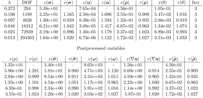
The iterations are terminated as soon as the relative error of the entire coefficient vectors between two consecutive iterates is small enough, that is. In our first example, we illustrate the accuracy of our method considering a manufactured exact solution defined on Ω considering the distribution of the boundary ΓN and ΓD=∂Ω\ΓN. We show in Tables 6.1 and 6.2 the convergence history for a sequence of quasi-uniform mesh refinements when the finite element spaces described in Section 4.1 are used with k = 0 and k = 1, respectively.
It can be observed there that the rates of convergence are those expected from theorem 5.2 and conclusion 5.3, respectively O(h) and O(h2). In Table 6.3, we summarize the convergence history for Example 2 considering a sequence of nearly uniform triangles. We observe there that the convergence rates O(h) predicted by Theorem 5.2 and Corollary 5.3 are all achieved for the unknowns and for all the post-processed variables.
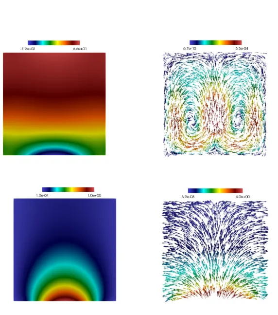
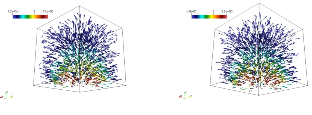
In addition, Figures 6.1, 6.2, and 6.3 compare the exact heat flux vector field, heat rate vector field, and temperature with their approximate counterparts. There we can see that the approximate solution satisfactorily captures the behavior of the exact solution. In our third example, we study the behavior of a liquid in a square cavity Ω = (0,1)2 with differently heated walls.
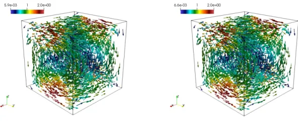
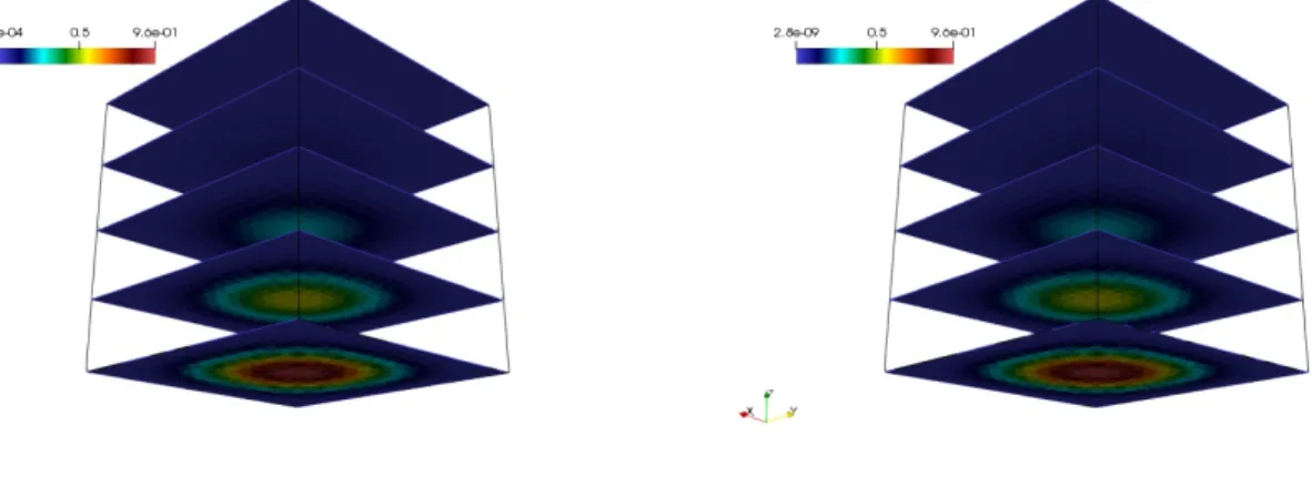
Here, since the analytical solution is unknown, we construct the convergence history by considering a solution computed with 1,161,246 DOF as the exact solution and using tolerancetol= 1e-6 and aRT0-P0-RT0-P0. In Figure 6.4, we show the approximated pressure and temperature (top left and bottom left, respectively) along with the approximated velocity and heat flux vector fields (top right and bottom right, respectively). There it is possible to see the expected physical behavior from [20], that is, convection currents are formed inside the cavity in a symmetric configuration, and due to the relatively low Rayleigh number, the heat transfer through the fluid is mainly due to conduction.
On the other hand, since the solution is smooth, it makes sense to expect convergence of O(h) when applying our method with k = 0; a fact that can be verified from the results in Table 6.4. In order to illustrate the conservative property of our method, we display in Table 6.5 the l∞ norm of divσh+gθh and divρh for the mixed RT0−P0−RT0−P0 approximation of the Boussinesq equations. Since divσh and gθh belong to Mh, it should be expected to obtain values close to zero for ∥divσh+gθh∥l∞ and similarly for ∥divρh∥l∞.
Moraga: A Banach space-based analysis of a new fully mixed finite element method for the Boussinesq problem. Das, Natural convection in a rectangular cavity heated from below and uniformly cooled from the top and both sides. Mitrea, Sobolev estimates the Green potential associated with the Robin-Laplacian in Lipschitz domains satisfying a uniform outer ball condition, Sobolev Spaces in Mathematics II, Applications in Analysis and Partial differential Equations.
Zúñiga, Analysis of a conformal finite element method for the Boussinesq problem with temperature dependent parameters. Creff, The steady Navier-Stokes/energy system with temperature-dependent viscosity - Part 2: The discrete problem and numerical experiments. Tagami, Error estimations of finite element methods for non-stationary thermal convection problems with temperature-dependent coefficients.
PRE-PUBLICACIONES 2019