Tensor Networks for Statistical Mechanics

(1)

Tensor Networks for Statistical Mechanics

Part I. 17:00 PM (Kobe), 22 Feb. 2021

Tomotoshi. Nishino (Kobe Universty)

Part II. 17:00 PM (Kobe), 24 Feb. 2021

Tensor network structure in statistical systems — [ Ising Model ]

Elementary algorithms for the calculation of partition functions (from Baxter)

Application examples (if there is some time)

ANNNI models (effect of frustration)

to higher dimension PEPS/TePS and TRG

Fractal lattices / Hyperbolic lattices

0 1 1 0 0 0 1 1 1 1 0 0 1 0 0 1

… HaPPY … Exotic systems:

Random-bond Ising model

(2)

why do I have to (?) speak about statistical mechanics?

to confirm that Quantum Mechanics is only a part of physics

“Strong correlation’’ also exists in statistical mechanics and other fields.

… but it is difficult of earn billions with the title “statistical …”

Tensor Network Structure is naturally contained in statistical systems.

(Path Integral representation of quantum systems)

Variational Formulation for a QM system “produces” a Statistical system.

(Most of the descriptions on TN are actually statistical.) just I love statistical physics,

from the time I had rich hair.

(3)

RE ^&' IT"KS OF MODERN PHYSIC& VOLUME 39, NUMBER ⁴ OCTOB F.R ^& ^&)ei ⁷

. .

^—.

, istory o): tIze . en' —. . sag .

^V.

. oc. e. .

STEPHEN G. BRIJSH

DePartment ofI'hysi cs and DePartment of^History ofScience, Harvard University, Cambridge, Massachusetts

Many physico-chemical systems can be represented more or less accurately by alattice arrangement of molecules with nearest-neighbor interactions. The simplest and most popular version of this theory is the so-called "Ising model,

"

_dis-

cussed by Krnst Ising ⁱⁿ 1925 but suggested earlier (1920) by ^Wilhelm Lenz.

Major events in the subsequent history of the Lenz—_Ising _model _are reviewed, including early approximate methods of solution, Onsager's exact result for the two-dimensional model, the use of the mathematically equivalent "lattice gas"

model to study gas—_liquid _and _liquid —solid phase transitions, and recent progress in determining the singularities of thermodynamic and magnetic properties at the critical point. Not only is there awide range ofpossible physical applications of the model, there is also an urgent need for the application of advanced mathematical techniques in order to establish its exact properties, especially in the neighborhood of phase transitions where approximate methods are un- reliable.

After _many years of being scorned or ignored by most scientists, the so-called "Ising model" has recently enjoyed increased popularity and may, if present trends continue, take its place as the preferred basic theory of all cooperative phenomena. Whereas previously it

appeared that the greatly over-simplified representation of intermolecular forces on which this model is based would make it inapplicable to any real systems, it is now being claimed that the essential features of cooperative phenomena (especially at the critical point) depend not on the details of intermolecular forces but on the mechanism of propagation of long-range order, and the Ising model ^is the only one which offers much hope of an accurate study of this mechanism. Whether or not it does eventually turn out that gas—_liquid _critical phenomena, magnetic Curie points, order—_disorder transitions in alloys, and phase separation in liquid mixtures can all be described, to a good first approxima- tion, by the same model, the problem of a generalized description of cooperative ^phenomena ^now ^deserves serious attention. We are just beginning to ^realize some of the implications of such a generalized description: specialists in the properties of gases and liquids could not afford to ignore progress being made in research on phase transitions in solids, and conversely.

While some scientists might not appreciate the burden imposed by the ^need for keeping up with the literature in unfamiliar fields which now suddenly appear to be related to ^their own, students should benefit by the prospective unification of different subjects. No longer would it be necessary to learn a different theory for

each kind of cooperative phenomenon.

The historical development of the "Ising model"

also shows the same disregard for traditional boundaries between disciplines. Physics, chemistry, metallurgy, and mathematics have all been involved, and some of the most recent applications have been in biology.

The most striking success in the history ^of the Ising model

—

the exact solution of the two-dimensional problem

—

^involved such difficult mathematics that it stumped all the physicists ^who attempted it, ^and ^was

8

finally accomplished by.

.

^.a ^chemist. (Just ^as ^ironical

is the fact that the supposed inventor of the model, Krnst Ising, gave up research in physics after thinking he had proved that his model had no physical useful- ness, and only discovered twenty years later that he had become famous as a result of work on his model by other scientists. )

THE MODEL

We assume that the physical system can be represented by a ^regular lattice arrangement of molecules in space. We are interested ⁱⁿ three kinds of physical systems: (1) ^magnets, ⁱⁿ ^which each molecule has a

"spin" that can be oriented either up or down relative to the direction of an externally applied field; (2) ^mix-

tures of two kinds of molecules; (3) ^mixtures ^of ^mole-

cules and "holes" _(empty _spaces)

.

^All three kinds can be represented abstractly by the same model, if we simply say that each node of a regular space lattice is assigned a ^two-valued ^variable. Depending on whether this variable has the value

+1

^or

—

_1, _we _say that the molecule at that ^node (1) ^has ^spin up or ^down, or (2)

belongs to one or the other of two species, (3) ^is ^present

or absent. Usually the two-valued variable is called the spiri ^o., ^associated ^{with node} i of the lattice.

A coegggraiioe of the lattice is a particular set of values of all the _spins; if there are

X

^nodes, ^there ^will

be 2~ different configurations. A typical configuration is shown in Fig. 1.

We assume that the molecules exert only short-range forces on each other; ⁱⁿ particular, we assume that the interaction energy depends only on the configurations of neighboring nodes of the lattice. For example, we could say that the forces are such that when two neighboring spins are the ^same (both

+1

^or ^both

—

₁₎ _the

energy is

—

_{U, and} _when two neighboring spins are different (one is

+1,

^{the other}

—

₁₎ the energy is

+U.

In other words, the interaction tends to make neighboring spins the same. In the three types of physical systems mentioned above, such an interaction could lead to (1) spontaneous magnetization, with all or

83

a century? of the Ising Model

W. Lenz, Phys. Z. 21, 613 (1920):

E. Ising, Z. 31, 253 (1925):

See Rev. Mod. Phys. 39, 883 (1967):

253

Beitrag zur Theorie des F e r r o m a g n e t i s m u s D.

Von Ernst Ising in Hamburg.

(Eingegangen am 9. Dezember 1924.)

Es wird im wesentlichen das thermische Verhalten eines linearen, aus Elementar- magneten bestehendea KSrpers untersueht, wobei im Gegensatz zur Weissschen Theorie des Ferromagaetismus keia molekulares Feld, somlern nur eine (nicht magnetisehe) Wechse[wirkung benachbarter Elemcatarmagnete aagenommeu wird.

Es wird gezeigt, dull tin sotehes Modell noch keine ferromagnetisehen Eigenschaften hcsitzt und diese Aussage auch auf das dreidimensionate )[odetl ausgedehnt.

1. A n n a h m e n . Die Erklarung, die P. W e i s s ~) ftir den Ferro- magneti~mus geg'eben hat, ist zwar formal befriedigend, doch Ial]t sie besanders die Frage nach einer physikalischen Erklarung der Hypothese des molekularen Fehles o[fen. Nach dieser Theorie wirkt au~ jeden E]ementarmagneten, abgesehen yon dem ~iul~eren 3[agnetfeld, ein inneres Fehl, das der ieweiligenMagne~isierungsinteasiti~t proportional ist. Es lieg't nahe. fiir die Wirkungen der einzelnen Elemente ( ~ Elementarmagnete) elektrische Dipolwirkungen anzuset, zen. Dann ergiiben sieh aber durch Summation der sehr langsam abnehmenden Dipolfelder sehr betrachtliche elektrische Feldst~rken, die dureh die Leitf~higkeit des Materials zerstSrt wCirden. Im Gegensatz zu P. W e i s s nehmen wir daher an, daft die Kr~ifte, die die Elemente atdeinander ausiiben, mit tier Entfernung raseh abklingen, so dal3 in erster N~herung sich nur benaehbarte Atome be-

einflussen.

Zweitens setzen wir an, dal~ die Elemente nur wenige der Kristall- , t r u k t u r entsprechende, energetiseh ausgezeichnete Orientierungen einnehmen. Infolge der W~rmebeweg'ung gehen die Elemente aus einer mggliehen Lage in eine andere tiber. W i r setzen an. dal~ die inhere Energie am kleins~en ist, wenn alle Elemente gleiehgerichtet sind. Diese Annahmen sind im wesentliehen zuerst yon W. L e n z s) aufgestellt und

n~her begrtindet worden.

2. D i e e i n f a c h e l i n e a r e K e t t e . Die gemaehtenVoraussetzungen wollen M r aM ein miiglichst einfaches Modell anwenden. W i t bereehnen das mittlere 3~oment $ e i n e s linearen 3lagneten, bestehend aus n Elemen~en.

.ledes dieser n Elemente soll nur die zwei Stellungen einnehmen ktinnen,

1) Auszug aus der Hamburger Dissertation.

'~) P. Weiss, Journ. de phys. (4) 6, 661, 1907, und Phys. ZS. 9, 358. 1908.

:~) W. Lenz, Phys. ZS. 21, 613, [920.

iSing and uSing

(4)

** Partition Function of 1D Ising Model is obtained as the trace of the products among transfer matrices T.

! e

^βJ

e

⁻^βJ

e

⁻^βJ

e

^βJ

" !

1

− 1

"

= 2 sinh βJ

! 1

− 1

"

. (2.18)

区別のために，式

(2.14)

の固有値を

λ

₀

= 2 cosh βJ ,

式

(2.18)

の固有値を

λ

₁

= 2 sinh β J

で表す．常に

λ

₀

> λ

₁ が満たされている．さて，関係式

! 1

0

"

= 1 2

! 1

1

"

+ 1 2

! 1

− 1

"

(2.19)

を式

(2.17)

に代入すると，分配関数

Z

^" が

Z

^"

= 1

2

# 2 cosh βJ $

N−1

+ 1 2

# 2 sinh βJ $

N−1

(2.20)

と求められることの確認は宿題にしておこう．

σ

₁ と

σ

_N が隣り合う周期境界条件では，式

(2.8)

に

T (σ

_N

| σ

₁

)

を付け加え

Z

^""

= %

σ₁···σ_N

T ( σ

₁

| σ

₂

) T ( σ

₂

| σ

₃

) · · · T ( σ

_N₋₁

| σ

_N

) T ( σ

_N

| σ

₁

) (2.21)

と分配関数を表せる．ダイアグラムに描いておこう．

1 2 N

式

(2.21)

は，転送行列

T

の

N

乗のトレースになっていて

Z

^""

= Tr T

^N

= #

2 cosh βJ $

N

+ #

2 sinh βJ $

N

(2.22)

と分配関数を求められる．

こうして，自由端条件の

Z

，固定端条件の

Z

^"，周期境界条件の

Z

^"" が，それぞれ「微妙に異なる」数式で表されることがわかった．この差異は，

N

が大きな極限では，あまり重要ではない．常に

cosh βJ > sinh βJ

が成立するので

N

lim

→∞

1 N

# − kT ln Z $

= lim

N→∞

1 N

# − kT ln Z

^"

$

= lim

N→∞

1 N

# − kT ln Z

^""

$

(2.23)

という具合に，スピン

1

個あたり（サイトあたり）の自由エネルギーが，境界条件に依存しないからである．

•

_{転送行列の}_{最大固有値}が，系の熱力学的な性質を決定する

というポイントを押さえておこう．少しだけ補足すると，最大固有値

λ

₀ _と，そ

の次に大きな固有値

λ

₁ の比

λ

₁

/λ

₀ が，スピン相関関数

" σ

_i

σ

_j

#

^の距離

| i − j |

に対する減衰を決定する．一般に，短距離の相互作用だけで記述される

1

次元の統計力学模型の場合，相関関数の減衰は常に指数関数的であって，相転移が起きることはない．ともかくも，大きい方から幾つかの転送行列固有値は，物理量に顔を出すという意味で，重要なものである．

2.2

転送行列の固有値

13

! e

^β^J

e

⁻^βJ

e

⁻^β^J

e

^βJ

" !

1

− 1

"

= 2 sinh βJ

! 1

− 1

"

. (2.18)

区別のために，式

(2.14)

の固有値を

λ

₀

= 2 cosh βJ ,

式

(2.18)

の固有値を

λ

₁

= 2 sinh β J

で表す．常に

λ

₀

> λ

₁ が満たされている．さて，関係式

! 1

0

"

= 1 2

! 1

1

"

+ 1 2

! 1

− 1

"

(2.19)

を式

(2.17)

に代入すると，分配関数

Z

^" が

Z

^"

= 1

2

# 2 cosh βJ $

N−1

+ 1 2

# 2 sinh βJ $

N−1

(2.20)

と求められることの確認は宿題にしておこう．

σ

₁ と

σ

_N が隣り合う周期境界条件では，式

(2.8)

に

T (σ

_N

| σ

₁

)

を付け加え

Z

^""

= %

σ₁···σ_N

T (σ

₁

| σ

₂

) T (σ

₂

| σ

₃

) · · · T (σ

_N₋₁

| σ

_N

) T (σ

_N

| σ

₁

) (2.21)

と分配関数を表せる．ダイアグラムに描いておこう．

1 2 N

式

(2.21)

は，転送行列

T

の

N

乗のトレースになっていて

Z

^""

= Tr T

^N

= #

2 cosh βJ $

N

+ #

2 sinh βJ $

N

(2.22)

と分配関数を求められる．

こうして，自由端条件の

Z

，固定端条件の

Z

^"，周期境界条件の

Z

^"" が，それぞれ「微妙に異なる」数式で表されることがわかった．この差異は，

N

が大きな極限では，あまり重要ではない．常に

cosh βJ > sinh βJ

が成立するので

N

lim

→∞

1 N

# − kT ln Z $ = lim

N→∞

1 N

# − kT ln Z

^"

$ = lim

N→∞

1 N

# − kT ln Z

^""

$ (2.23)

という具合に，スピン

1

個あたり（サイトあたり）の自由エネルギーが，境界条件に依存しないからである．

•

_{転送行列の}_{最大固有値}が，系の熱力学的な性質を決定する

というポイントを押さえておこう．少しだけ補足すると，最大固有値

λ

₀ と，その次に大きな固有値

λ

₁ の比

λ

₁

/λ

₀ が，スピン相関関数

" σ

_i

σ

_j

#

^の距離

| i − j |

に対する減衰を決定する．一般に，短距離の相互作用だけで記述される

1

次元の統計力学模型の場合，相関関数の減衰は常に指数関数的であって，相転移が起きることはない．ともかくも，大きい方から幾つかの転送行列固有値は，物理量に顔を出すという意味で，重要なものである．

2.2

転送行列の固有値

13

corresponding diagram (under periodic boundary condition)

Z = !

!

e

⁻^βE^!

(2.2)

は分配関数と呼ばれる．ここまで暗記すれば，統計力学は免許皆伝である．

【磁性体と相転移】

物質が関係する熱的な物理現象で，よく知られているものが氷の融解や水の沸騰などの相転移現象である．鉄の玉を引きつけた磁石を，ゆっくり加熱すると，ある温度でポロリと玉が落ちる．温度が上がると，磁石ではなくなるのだ．磁石を構成する物質（磁性体）は，低温では磁力を持った強磁性状態（強磁性相）にあり，相転移温度

T

_c を境に，それよりも高温では磁力を失った常磁性状態（常磁性相）となる．このような変化を磁性相転移と呼ぶ．

磁性体では，原子がそれぞれ小さな磁石としての働きを受け持っている^∗¹^）．この原子磁石が，どうして同じ向きにそろっているの

?

という素朴な疑問を，

モデル化して簡単な数式に落としたものがイジング模型である．原子磁石が並んだ状態を思い浮かべて，（

N

極が）上向きの状態を

σ = 1

で，下向きの状態を

σ = − 1

で表現する．単純化するのが目的なので，それ以外の向きは考えない^∗²^）．原子磁石の向きは，原子が持つスピン角運動量に起因しているので，この

σ

をイジングスピン，あるいは単にスピンと呼ぶ習慣がある．

図 2.1 上向きが σ_i = 1，下向きが σ_i = −1

図

2.1

のように原子磁石を表すスピン

N

個が一列に並んだ系を考えよう．

小さな白丸で示したスピンに番号を振って，左からそれぞれ

σ

₁

, σ

₂

, · · · , σ

_N で表すことにする．

i

番目のスピンは

σ

_i だ．原子磁石間に，量子力学的な過程に起因する相互作用が働いて，隣り合う原子磁石が同じ向きの場合にエネルギーが低くなる場合を考える（逆向きであれば，エネルギーは高くなる）．隣り合うスピン

σ

_i と

σ

_i+1 の間の相互作用エネルギーを

− J σ

_i

σ

_i+1 と表すと，

この状況を記述できる．

J > 0

は相互作用の強さを表すパラメターだ．相互作用を合計したものが，

1

次元イジング模型のハミルトニアン

H = − J "

σ

₁

σ

₂

+ σ

₂

σ

₃

+ · · · + σ

_N₋₁

σ

_N

#

= − J

N

!

−1 i=1

σ

_i

σ

_i+1

(2.3)

である．スピンが全て上向き

σ

_i

= 1

ならば

H = − (N − 1)J

で，これがエネルギーの最小値である．一方，最大値は

H = (N − 1)J

で，これはスピンが

*1）こういういい加減な説明をすると，磁性の研究者から沢山の突っ込みを受ける．物質が磁石になる理由は様々あって，ここで紹介したのはホンの入り口に過ぎない．後は専門家に任せよう．

*2）用語としての向きと方向は，高校物理では区別して使われているらしい．

2.1 1 次元イジング模型と転送行列 9

Ising Spin: up (1) and down (-1) Hamiltonian

Z = !

!

e

⁻^β^E^!

(2.2)

は分配関数と呼ばれる．ここまで暗記すれば，統計力学は免許皆伝である．

【磁性体と相転移】

物質が関係する熱的な物理現象で，よく知られているものが氷の融解や水の沸騰などの相転移現象である．鉄の玉を引きつけた磁石を，ゆっくり加熱すると，ある温度でポロリと玉が落ちる．温度が上がると，磁石ではなくなるのだ．磁石を構成する物質（磁性体）は，低温では磁力を持った強磁性状態（強磁性相）にあり，相転移温度

T

_c を境に，それよりも高温では磁力を失った常磁性状態（常磁性相）となる．このような変化を磁性相転移と呼ぶ．

磁性体では，原子がそれぞれ小さな磁石としての働きを受け持っている^∗¹^）．この原子磁石が，どうして同じ向きにそろっているの

?

という素朴な疑問を，

モデル化して簡単な数式に落としたものがイジング模型である．原子磁石が並んだ状態を思い浮かべて，（

N

極が）上向きの状態を

σ = 1

で，下向きの状態を

σ = − 1

で表現する．単純化するのが目的なので，それ以外の向きは考えない^∗²^）．原子磁石の向きは，原子が持つスピン角運動量に起因しているので，この

σ

をイジングスピン，あるいは単にスピンと呼ぶ習慣がある．

図

2.1

上向きが

σ

_i

= 1

，下向きが

σ

_i

= − 1

図

2.1

のように原子磁石を表すスピン

N

個が一列に並んだ系を考えよう．

小さな白丸で示したスピンに番号を振って，左からそれぞれ

σ

₁

, σ

₂

, · · · , σ

_N

で表すことにする．

i

番目のスピンは

σ

_i だ．原子磁石間に，量子力学的な過程に起因する相互作用が働いて，隣り合う原子磁石が同じ向きの場合にエネルギーが低くなる場合を考える（逆向きであれば，エネルギーは高くなる）．隣り合うスピン

σ

_i と

σ

_i+1 の間の相互作用エネルギーを

− J σ

_i

σ

_i+1 と表すと，

この状況を記述できる．

J > 0

は相互作用の強さを表すパラメターだ．相互作用を合計したものが，

1

_{次元イジング模型}のハミルトニアン

H = − J "

σ

₁

σ

₂

+ σ

₂

σ

₃

+ · · · + σ

_N₋₁

σ

_N

# = − J

N

!

−1 i=1

σ

_i

σ

_i+1

(2.3)

である．スピンが全て上向き

σ

_i

= 1

ならば

H = − ( N − 1) J

で，これがエネルギーの最小値である．一方，最大値は

H = (N − 1)J

で，これはスピンが

*1）こういういい加減な説明をすると，磁性の研究者から沢山の突っ込みを受ける．物質が磁石になる理由は様々あって，ここで紹介したのはホンの入り口に過ぎない．後は専門家に任せよう．

*2）用語としての向きと方向は，高校物理では区別して使われているらしい．

2.1 1

次元イジング模型と転送行列

9

this is an example of tensor network, which is formed by

the contraction among two-leg tensors, the transfer matrices T.

(5)

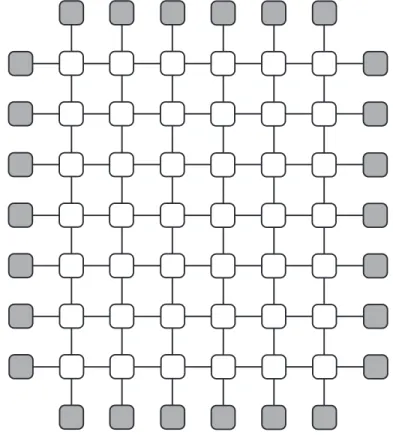
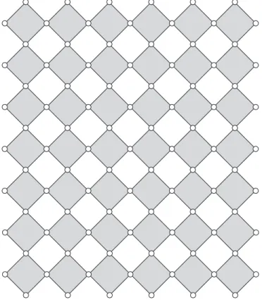
2D Ising model on Diagonal Lattice

2.3 2 次元イジング模型のテンソルネットワーク表現

今度はスピンが 2 次元的に並んだ

正方格子イジング模型

を例に取ろう．碁盤や障子のような格子を考えるのだけれども，後に続く数式などを単純にするため，図 2.2 に描いたような格子 — 対角格子 (diagonal lattice) — を考える．小さな白い丸が ± 1 の値を取るスピンを表し，斜めの実線で結ばれたスピン間には，イジング相互作用 − J σσ

^!

が働いている．説明の都合で， 4 つのスピンが囲む正方形を「一つおき」に薄く灰色に塗っておく．灰色の正方形が横に並ぶ数を N ，縦に積み重なる数（段数）を M としよう．スピンの総数は N (M + 1) + (N + 1)M 個である．図には N = 6, M = 7 の場合を示してある．分配関数を表していこう．

図

2.2

横に

N = 6

個，縦に

M = 7

個，灰色の正方形を並べたもの

スピンに

位置のラベル

を付けよう．まず，最下部に並ぶ N 個を

σ

₁⁽⁰⁾

, σ

₂⁽⁰⁾

, · · · , σ

_N⁽⁰⁾₋₁

, σ

_N⁽⁰⁾

(2.24)

で表す． σ

_i⁽⁰⁾

の肩に置いた

⁽⁰⁾

は “0 段目 ” であることを示している．最下段に並ぶ灰色の正方形と，「一つ上の段」に並ぶ灰色の正方形が共有している N 個のスピンは σ

₁⁽¹⁾

, σ

₂⁽¹⁾

, · · · , σ

_N⁽¹⁾

で表し，段ごとに肩文字を増やしていく．

縦に M 段，灰色の正方形を積んであるので，いちばん上に並ぶ N 個のスピ

ンは σ

₁⁽^M⁾

, σ

₂⁽^M⁾

, · · · , σ

_N⁽^M⁾

となる．まだ，ラベル付けされていないスピンが

(N + 1)M 個，残っている．最下段に並ぶ灰色の正方形について，それぞれの

左右に位置するスピンを，左から

s

⁽¹⁾₀

, s

⁽¹⁾₁

, s

⁽¹⁾₂

, · · · , s

⁽¹⁾_N₋₁

, s

⁽¹⁾_N

(2.25)

と表そう．今度は肩文字を

⁽¹⁾

から始め，段ごとに肩文字を増やし，最上段に並ぶ正方形の左右に位置するスピンは s

^(M₀ ⁾

, s

^(M₁ ⁾

, s

^(M₂ ⁾

, · · · , s

^(M_N ⁾

と表す．このように 2 種類の文字を導入した理由は， σ

_i^(j)

が縦に積み重なる正方形の接続部分にあり， s

^(j)_i

が横に並ぶ正方形の間にあって，働きが異なるからである．

14

第

2

章統計力学とテンソルネットワーク

式

(2.26)

に示した，灰色の正方形のエネルギーに対応する，局所的なボル

ツマン重率

W

_i^(j)

= exp ! J kT

"

σ

_i^(j⁻¹⁾

s

^(j)_i₋₁

+ s

^(j)_i₋₁

σ

_i^(j)

+ σ

_i^(j)

s

^(j)_i

+ s

^(j)_i

σ

_i^(j⁻¹⁾

#$

(2.29)

を導入しよう．その値が次のとおりであることを，地道に確認しておくとよい．

• 4

つのスピンが同じ向き（同じ値）の場合には

e

^4J/kT

• 1

つだけ逆向き（異なる値）の場合には

e

^0/kT

= 1

• σ

_i^(j⁻¹⁾

= σ

_i^(j) 及び

s

^(j)_i₋₁

= s

^(j)_i で，

σ

_i^(j)

! = s

^(j)_i の場合には

e

⁻^4J/kT

W

_i^(j) は，

4

つのスピン

—

左右に

s

^(j)_i₋₁ と

s

^(j)_i ，上下に

σ

_i^(j) と

σ

_i^(j⁻¹⁾

—

を脚に持つテンソルとみなせる．ダイアグラムで表しておこう．

j-1 j

i-1 i

テンソルの脚を表す「突き出た線」の先に，何を添え書きするかは，場合によりけりで，何も書かないこともあれば，脚に対応する変数を書き込むこともある．ここでは，縦横の位置を書き込んだ．この図形を使って式

(2.28)

の分配関数を表すダイアグラムを描くと，次のような図形になる．

図 2.3 分配関数を表すダイアグラム．灰色の 1 脚テンソルは自由境界条件を示す．

テンソルの縮約が網目を作って，ようやくテンソル_ネ

˙

_ッ

˙

_ト

˙

_ワ

˙

_ー

˙

_{クらしくなっ}

˙

てきた．

1

次元イジング模型の場合と同じように，境界のスピンについての和は，値が常に

1

である

1

脚テンソルとの縮約と解釈して，灰色の図形で示した．具体的には，左側に縦に並ぶ

L "

σ

₀^(j)

#

，右側の

R "

σ

^(j)_N

#

，下側の

D %

σ

_i⁽⁰⁾

&

，上側の

U %

σ

_i^(M⁾

&

が，境界での縮約を記述する（これら，境界に並ぶテンソルの値を変更すると，異なる境界条件を課すことができる）．

16 第 2 章統計力学とテンソルネットワーク

i-1 i i

j-1 j j

今度は灰色の正方形それぞれに着目しよう．下から j 段目（j = 1,2,· · ·, M）

左から i 番目（i = 1,2,· · ·, N）に位置する灰色の正方形は，4 つのスピン

σ_i^(j)

s^(j)_i₋₁ s^(j)_i σ_i^(j⁻¹⁾

に囲まれている（上図参照）．上下左右の順でスピン

を並べると，σ_i^(j⁾, σ_i^(j⁻¹⁾ と s^(j)_i₋₁, s^(j_i ⁾ となる．イジング模型では，隣り合うスピンが同じ値（同じ向き）であれば相互作用エネルギーが −J に，異なる値

（逆向き）であれば J になるのであった．従って，いま着目している 4 つのスピン間のイジング相互作用は 4 項の和

−J σ_i^(j⁻¹⁾s^(j)_i₋₁− J s^(j)_i₋₁σ_i^(j) −J σ_i^(j)s^(j)_i −J s^(j)_i σ_i^(j⁻¹⁾ (2.26) になる．これを，格子全体にわたって足し合わせたものが，この章の主役である 2 次元イジング模型のハミルトニアンである．

H =

!N i=1

!M j=1

"

−J#

σ_i^(j⁻¹⁾s^(j)_i₋₁+s^(j)_i₋₁σ_i^(j⁾+σ_i^(j)s^(j_i ⁾+s^(j)_i σ_i^(j⁻¹⁾$%

.(2.27) これに対応するボルツマン重率は exp&

H kT

'

であり，式 (2.7) と同様に，あらゆるスピン配列について和を取ると，温度 T での分配関数を表す式

Z = !

{σ}

!

{s}

exp&

H kT

' (2.28)

となる．全ての σ_i^(j) を {σ} ^{と，全ての} s^(j)_i を{s} ^{と略記して総和記号} ( _の下に置いた．境界に位置する 2N + 2M 個のスピンについても和を取っているので，自由境界条件を設定したことになっている．

【熱力学極限】

水や磁石など，十分に多数の原子を含む物質の巨視的な性質を説明するためには，構成要素である原子の数や物質の体積などが十分に大きな場合を取り扱わなければならない．これは熱力学極限と呼ばれる，統計物理学で重要な概念だ．式 (2.28) に書き下した分配関数では，N や M が十分に大きな場合を取り扱うこと，つまり N → ∞, M → ∞ の極限を意味する．物質の相転移現象を議論する際には，熱力学極限を取った上で解析する必要がある．境界の効果が見えなくなるまで大きくする，と考えても良いだろう．対象となる物理系を支配する相互作用が短距離のものであれば，比較的小さな系でも熱力学極限と同じ性質を示す．

2.3 2 次元イジング模型のテンソルネットワーク表現 15

式 (2.26) に示した，灰色の正方形のエネルギーに対応する，局所的なボル

ツマン重率

W_i^(j) = exp! J kT

"

σ_i^(j⁻¹⁾s^(j)_i₋₁ +s^(j)_i₋₁σ_i^(j) +σ_i^(j)s^(j)_i +s^(j)_i σ_i^(j⁻¹⁾#$

(2.29)

•4 つのスピンが同じ向き（同じ値）の場合には e^4J/kT

•1 つだけ逆向き（異なる値）の場合には e^0/kT = 1

•σ_i^(j⁻¹⁾ = σ_i^(j) 及び s^(j)_i₋₁ = s^(j)_i で，σ^(j)_i != s^(j)_i の場合には e⁻^4J/kT

W_i^(j) は，4 つのスピン — 左右に s^(j)_i₋₁ と s^(j)_i ，上下に σ_i^(j) と σ_i^(j⁻¹⁾ — を脚に持つテンソルとみなせる．ダイアグラムで表しておこう．

j-1 j

i-1 i

テンソルの脚を表す「突き出た線」の先に，何を添え書きするかは，場合によりけりで，何も書かないこともあれば，脚に対応する変数を書き込むこともある．ここでは，縦横の位置を書き込んだ．この図形を使って式 (2.28) の分配関数を表すダイアグラムを描くと，次のような図形になる．

図 2.3 分配関数を表すダイアグラム．灰色の 1 脚テンソルは自由境界条件を示す．

テンソルの縮約が網目を作って，ようやくテンソル_ネ˙ _ッ˙ _ト˙ _ワ˙ _ー˙ _{クらしくなっ}˙ てきた．1 次元イジング模型の場合と同じように，境界のスピンについての和は，値が常に 1 である 1 脚テンソルとの縮約と解釈して，灰色の図形で示した．具体的には，左側に縦に並ぶ L"

σ₀^(j)#

，右側の R"

σ_N^(j)#

，下側の D%

σ_i⁽⁰⁾&

，上側の U%

σ_i^(M⁾&

式 (2.26) に示した，灰色の正方形のエネルギーに対応する，局所的なボル

ツマン重率

W_i^(j) = exp! J kT

"

σ_i^(j⁻¹⁾s^(j)_i₋₁+s^(j)_i₋₁σ^(j)_i +σ_i^(j)s^(j)_i +s^(j)_i σ_i^(j⁻¹⁾#$

(2.29)

•4 つのスピンが同じ向き（同じ値）の場合には e^4J/kT

•1 つだけ逆向き（異なる値）の場合には e^0/kT = 1

•σ^(j−1)_i = σ_i^(j) 及び s^(j)_i−1 = s^(j)_i で，σ^(j)_i != s^(j)_i の場合には e^−4J/kT W_i^(j) は，4 つのスピン — 左右に s^(j)_i−1 と s^(j)_i ，上下に σ_i^(j) と σ_i^(j−1) — を脚に持つテンソルとみなせる．ダイアグラムで表しておこう．

j-1 j

i-1 i

テンソルの脚を表す「突き出た線」の先に，何を添え書きするかは，場合によりけりで，何も書かないこともあれば，脚に対応する変数を書き込むこともある．ここでは，縦横の位置を書き込んだ．この図形を使って式 (2.28) の分配関数を表すダイアグラムを描くと，次のような図形になる．

図2.3 分配関数を表すダイアグラム．灰色の 1 脚テンソルは自由境界条件を示す．

テンソルの縮約が網目を作って，ようやくテンソル_ネ˙ _ッ˙ _ト˙ _ワ˙ _ー˙ _{クらしくなっ}˙ てきた．1 次元イジング模型の場合と同じように，境界のスピンについての和は，値が常に 1 である 1 脚テンソルとの縮約と解釈して，灰色の図形で示した．具体的には，左側に縦に並ぶL"

σ₀^(j)#

，右側の R"

σ_N^(j)#

，下側の D% σ_i⁽⁰⁾&

，上側の U%

σ^(M_i ⁾&

16 第2章統計力学とテンソルネットワーク

shaded square: interaction among 4 spins

corresponding Boltzmann weight

Partition Function: 2D Tensor Network

one-leg tensors represent the boundary conditions.

Putting Ising spins on the diagonal lattice, and

putting local Boltzmann weights for shaded squares.

(6)

Tensor Network structure naturally emerges from the lattice statistical models.

表現することは難しいので，数式を書く人ごとに，それどころかページ毎に，

省略の方法が変わるような事例にもよく接する．式

(2.30)

を更に

!

s^(j)_i

W

_i^(j)

W

_i+1^(j)

= X

とか，単に

W

_i^(j)

W

_i+1^(j⁾

= X (2.33)

と略記することも可能だし，このような記述もよく使われる（以下でバンバン使う

!

）．結局のところ，数式に頼る限り誤解を避けることは難しいので，ダイアグラムという共通語の利用が一般的となっている．

図 2.4 転送行列を表すダイアグラム：左端は L

"

s⁽₀^j⁾

#

，右端は R

"

s⁽_N^j⁾

#

図

2.4

のように，

j

段目のテンソル

W

₁^(j)

, · · · , W

_N^(j⁾ と，自由端条件を表すテンソル

L "

s

^(j)₀

#

= 1, R "

s

^(j_N⁾

#

= 1

の間で，

s

^(j)₀

, s

^(j)₁

, · · · s

^(j_N⁾ について縮約を取ったものを考えよう．略記した形の数式で表すと

T

^(j⁾

= !

{s^(j)}

L W

₁^(j⁾

W

₂^(j)

· · · W

_N^(j)

R (2.34)

となる．横一列に並ぶスピンの列を示す目的で，和記号の下に

{ s

^(j)

}

^という

「まとめ書き」を使った^∗⁵^）．

T

^(j⁾ は，

2

次元イジング模型の転送行列で，

T

^(j⁾ の要素を省略せずに表すと^∗6^）

T

$ % σ

^(j⁾

&

% σ

^(j⁻¹⁾

&

'

= T

$ σ

₁^(j)

σ

₂^(j)

· · · σ

_N^(j)

σ

₁^(j⁻¹⁾

σ

₂^(j⁻¹⁾

· · · σ

^(j_N⁻¹⁾

'

(2.35)

となる左辺では，

T

^(j) の上下に並ぶスピンの列を「まとめ書き」してある．転送行列

T

^(j⁾ は

2

^N 次元の行列で，その基本的な働きは前節の式

(2.6)

で考えた

1

次元イジング模型の転送行列と同じである．転送行列

T

^(j⁺¹⁾ と

T

^(j) の積をダイアグラムで表すと，次のように縦に並べて，

間にある

{ σ

^(j)

}

について縮約を取ったものとなる．数式で表すと

Q

$ % σ

^(j⁺¹⁾

&

% σ

^(j⁻¹⁾

&

'

= !

{σ^(j⁾}

T

$ % σ

^(j⁺¹⁾

&

% σ

^(j⁾

&

' T

$ % σ

^(j⁾

&

% σ

^(j⁻¹⁾

&

'

(2.36)

*5） L や R をベクトルと，W_i^(j) を行列とみなし，右辺の総和記号を省略する表記もよく見かける．本書では，可能な限り，総和記号の省略を避けるつもりだ．

*6）用語として，テンソルとテンソルの要素は，あまりハッキリと区別されない場合が多い．これは行列でも同じで，「単位行列 I_ij = δ_ij」などという記述も稀ではない．

To obtain the largest eigenvalue of the transfer matrix (precisely), when the system width N is large enough, is a main purpose of numerical

calculation. Variational estimation is often considered.

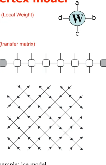
Vertex model a

b c

d W

example: ice model

Lieb, Phys. Rev. 162, 162 (1967)

(Local Weight)

2^N-dimensional real (symmetric)

(transfer matrix)

(7)

PHYSI ^CAL REVIEW ^VOLUME 113, NUMBER ⁴ FEBRUARY 15, 1959

Transformations of Ising Models

MxcHAEx. K. FxsHKR

Wheatstone Physics Laboratory, Zing's College, London, England (Received August 29, 1958)

The "star-triangle" and "decoration" transformations are generalized soas toapply toarbitrary ^mechani- cal systems coupled to the spins ofastandard Ising net. This leads to exact solutions for further plane Ising nets and also forlattices in which the spins on alternate sites have amagnitude greater than S=^—,.^{A general}

class of antiferromagnetic Ising models is constructed; exact closed expressions can be derived for all the thermodynamic and magnetic properties of these models in an arbitrary magnetic field.

The magnetizations and susceptibilities of Ising nets in which different spins have different magnetic moments are investigated and a valuable relation between the susceptibilities of the honeycomb and tri- angular lattices is derived. It<

Tensor Networks for Statistical Mechanics