Testing for the General Fractional Unit Root Hypothesis in the Time Domain

(1)

TESTING FOR THE GENERAL FRACTIONAL UNIT ROOT HYPOTHESIS IN THE TIME DOMAIN

UWE HASSLER

PAULO M.M. RODRIGUES ANTONIO RUBIA

FUNDACIÓN DE LAS CAJAS DE AHORROS DOCUMENTO DE TRABAJO

Nº 380/2008

(2)

De conformidad con la base quinta de la convocatoria del Programa de Estímulo a la Investigación, este trabajo ha sido sometido a eva- luación externa anónima de especialistas cualificados a fin de con- trastar su nivel técnico.

La serie DOCUMENTOS DE TRABAJO incluye avances y resultados de investigaciones dentro de los pro- gramas de la Fundación de las Cajas de Ahorros.

Las opiniones son responsabilidad de los autores.

(3)

Testing for the General Fractional Unit Root Hypothesis in the Time Domain

Uwe Hassler

^a

, Paulo M.M. Rodrigues

^b

and Antonio Rubia

^c

a Goethe University Frankfurt b University of Algarve c University of Alicante

March 2008

Abstract

In this paper we propose a Lagrange Multiplier test as well as a family of asymptotically equivalent LS-based testing procedures which are intended to detect general forms of fractional integration at the long-run and/or the cyclical component of a time series.

Our setting extends Robinson´s (1994) approach to the time domain and generalizes the procedures in Agiakloglou and Newbold (1994), Tanaka (1999) and Breitung and Hassler (2002) by allowing for single or multiple fractional unit roots at any frequency in [0; ]. Our testing procedure can be easily implemented in practical settings and is ‡exible enough to account for a broad family of long- and short-memory speci…cations, including ARMA-type and/or GARCH-type dynamics, among others. Furthermore, it has power against di¤erent types of alternative hypotheses and inference is conducted under critical values drawn from a standard chi-squared distribution, independently of the long-memory parameters.

Keywords: LM tests, nonstationarity, fractional integration, cyclical integration JEL classi…cation: C20, C22

Acknowledgement: The authors thank Peter Phillips, Luis A. Gil-Alaña, Javier Hualde, and the partic- ipants of the conference in Honour of Paul Newbold, University of Nottingham, and seminar attendants at the University of Navarra and University of Évora for useful comments and suggestions. Financial support from POCTI/ FEDER (grant ref. PTDC/ECO/64595/2006), SEJ2005-09372/ECON project (Spanish Department of Education and Science), and GRJ0613 project (University of Alicante) is gratefully acknowledged.

(4)

1 Introduction

Modelling and forecasting macroeconomic and …nancial variables is at the forefront of the applied time-series econometric literature. These series are usually characterized by strongly persistent correlation structures over long intervals of time. In this paper, we propose several test statistics to detect general forms of fractional integration in the time domain. Our approach be- longs to the Lagrange-multiplier (LM) framework studied in Robinson (1991, 1994), Agiakloglou and Newbold (1994), Tanaka (1999), Breitung and Hassler (2002) and Nielsen (2004, 2005). In particular, we propose standard LM tests for multiple fractional integration, as well as a family of asymptotically equivalent tests in the linear regression modelY_t=Pn

s=1 sX_st(Y_t)+u_t, where Y_t is directly determined under the null hypothesis and the regressors X_st(Y_t) are straightforwardly computed by linearly …lteringYt:This approach has remarkable methodological advan- tages. It can be easily implemented for practical settings and is ‡exible enough to account for a broad family of long- and short-memory speci…cations. Furthermore, it also has power against di¤erent types of alternative hypotheses, and it allows inference to be conducted under critical values which are drawn from a standard chi-squared distribution, independently of the long-memory parameters.

More speci…cally, the tests we discuss are formally intended to detect general long memory patterns embedded in the autoregressive …lter

(1 L)^d¹

"_k+1 Y

i=2

(1 2 cos _iL+L²)^dⁱ

#

(1 +L)^d^k+2

where d_i; i = 1; :::; k+ 2; are possibly non-integer values, _i, 1 i k+ 1, are frequencies in (0; )that characterize the cyclical behavior (periodicity) of the data, andLis the conventional back-shift operator. The …lter also allows for long-memory patterns at the zero and Nyquist frequencies. This is the basic data generating process analyzed in Robinson (1994), which is able to capture both long-range dependence and periodic cyclical ‡uctuations through the convolution of Gegenbauer processes. It generates theoretical autocovariances that decay hyperbolically and sinusoidally, a feature that is manifested in a number of periodic time series. Particular cases of this speci…cation include the well-known fractional unit root model, as well as pure cyclical and seasonal models which are routinely applied to …t both economic and non-economic variables.

For instance, cyclical models have been used to explain macroeconomic dynamics by Gray, Zhang and Woodward (1989), Ramachandran and Beaumont (2001), Gil-Alana and Robinson (2001), Gil-Alana (2005), and Smallwood and Norrbin (2006), among many others. Recent studies focusing on non-economic variables have analyzed, for instance, atmospheric levels of CO2 (Woodward, Cheng and Gray, 1998), wind speed (Bouetteet al:, 2006), or power demand (Soares and Souza, 2006). The extant literature on seasonal and non-seasonal models embedded in this general framework (both integrated and fractionally integrated) is overwhelming.

Our setting extends Robinson’s approach to the time domain and generalizes the procedures in Agiakloglou and Newbold (1994), Tanaka (1999) and Breitung and Hassler (2002) by allowing for single or multiple fractional unit roots at any frequency in [0; ]. Furthermore, we allow for di¤erent types of errors in the data generating process (DGP) which include martingale di¤erences sequences (MDS) and weakly correlated errors, thus allowing for ARMA and/or time varying volatility patterns. As in the frequency-domain case, the tests do not

(5)

require formal knowledge of the true values of the fractionally-integrated coe¢ cients. These are mainly intended for formally pretesting hypotheses about the extent of cyclical and non-cyclical persistence, and to construct con…dence sets that include the true values of the long-memory coe¢ cients with a certain asymptotic coverage level. This is valuable for descriptive inference and, furthermore, provides reliable values for initiating optimization routines upon which several estimation procedures, such as (quasi) maximum likelihood procedures, build on.

The remaining of the paper is organized as follows. Section 2 introduces the general setting and discusses the set of su¢ cient conditions for the LM tests. Section 3 introduces the standard Lagrange Multiplier test and discusses its asymptotic distribution. Section 4 discusses regression-based tests. The speci…c form of the regression to be used depending on the type of errors in the DGP, the relevant test statistics, and their asymptotic distributions, is discussed in several theorems. Section 5 analyzes the …nite-sample performance of the tests by means of Monte Carlo experimentation. Section 6 summarizes the main conclusions. Finally, the mathematical proofs of the main statements are collected in a technical appendix.

In what follows, ‘)’ and ‘!^p ’ denote weak convergence and convergence in probability, respectively, as the sample size is allowed to diverge. The variable I^{( )} is an indicator function that takes value equal to one if the condition in the subscript is ful…lled and zero otherwise.

Finally, vectors and matrices are denoted through bold letters.

2 The general fractionally integrated model

Let (L; ) be a Gegenbauer polynomial in the lag operator de…ned as follows,

(L; ) = (1 2 cos L+L²) (1)

where the long-memory parameter can take non-integer values and controls the extent of time dependence. The parameter is a so-called Gegenbauer frequency in [0; ]; and controls the periodicity of the resulting time series.

De…ne the following generalization of (1); given the set of long-memory parameters = ( ₁; :::; _k+2)⁰; 2R^k+2; and the vector of frequencies = ₁; :::; _k+2 ⁰

(L; ) (1 L) ¹

"_k+1 Y

i=2

i(L; _i)

#

(1 +L) ^k+2 (2)

such that ₁ < ₂ < < _k+2;and by de…nition ₁ = 0; _k+2 = . The resultant …lter allows for multiple cyclical components for thek+ 1seasonal frequencies involvedf s :s >1g, as well as for a long-run trend at the zero frequency, ₁. For simplicity of notation, the dimension of is denoted as n 1. Speci…cation (2) encompasses di¤erent types of …lters. In addition to the well-known fractionally integrated unit-root model, major examples for empirical purposes include pure cyclical models (which arise by restricting ), pure seasonal models (which arise by restricting ), and any convolution of these. We shall brie‡y discuss the properties of these restricted models at the end of this section.

We consider that the observable process, fx_t; t= 1; :::; Tg, admits the following character- ization

(L; )x_t="_t (3)

(6)

where "_t is a covariance stationary noise process with spectral density that is bounded and bounded away from zero at all frequencies. In the most general case considered in this paper, we will say thatx_t is generated by aGeneral Fractionally Integrated process of order ;denoted as x_t GFI( ): The study of particular cases (such as zero frequency, seasonal models, and cyclical models) arises straightforwardly by suitably restricting (L; ). For instance, pure cyclical models arise by restricting and setting the long-memory parameters corresponding to the zero and Nyquist frequencies to zero. The restricted …lter isQn

i=1 i(L; _i);with dimension n 1:Whenn = 1,x_t is said to be generated by a GARMA model, whereasn > 1leads to so- calledn-factor GARMA models, which exhibit stationary long-memory patterns if0< _i <1=2;

see Woodward et al. (1998), and Ramachandran and Beaumont (2001) for a discussion of the statistical properties of these models. The generalizations (for instance, allowing for stationary short-run dynamics) are able to encompass both ARMA and ARFIMA models as particular cases.

Similarly, pure seasonal models (SARFIMA) arise by restricting both the dimension and the value of aiming to relate the frequencies to the periodicity of the data, sayS. For instance, if S is even, then ₁ = 0 and _i+1 = 2 i=S; i = 1; :::;[S=2] 1, where the corresponding …lter is now given by

(1 L) ¹ 2 4

[S=2] 1Y

i=2

i(L; i) 3

5(1 +L) ⁿ (4)

with dimensionn = [S=2] + 1:WhenS is odd, the component(1 +L) ⁿ;which corresponds to a cycle of two periods, is simply omitted and the model has[S=2]parameters. A special case is

1 =:::= _n= 1;from which the …lter 1 L^S originating a seasonal random walk arises. By allowing non-integer values in ; xt is said to be generated by a seasonal fractionally integrated process of order ; see, among others, Hassler (1994) and references therein.

Finally, the well-known fractional unit root model of order d, denoted FI(d); arises after removing all the terms related to the non-zero frequencies, i:e:, by considering the (1 L)^d

…lter related to the zero frequency = 0, which corresponds to the ARFIMA(0,d,0) model.

For empirical purposes, the main interest lies in testing whether =d; with d2Rⁿ being speci…ed a priori, against the alternative for which the order of integration is d+ ; 6= 0:

Thus, the hypothesis of interest is generally stated as

H0 : =d;or H0 : =0; (5)

against the alternative hypothesis that H0 is false, i.e., H1 : 6=d or H1 : 6=0:

3 Testing procedures

3.1 Preliminaries

We start our theoretical analysis by introducing and discussing the initial set of assumptions and general notational issues which are valid for both the standard LM and the regression-based tests. We also provide several key de…nitions for this context.

(7)

Assumption A:

i)The observable process fx_t; t= 1; :::; Tgis generated by (L;d)x_t="_tI^(t>0), with (L;d) de…ned in (2); and d being a possibly non-integer vector in Rⁿ; n 1:

ii) The innovation process f"_t;G^tg¹₁; G^t = ("_j :j t); forms a martingale di¤erence se- quence and veri…es E ("_t) = 0; E("²_t) = ² <1; E("²_tjG^t ¹)>0almost surely, with one of the following restrictions holding true:

ii:a) f"_tg is independent and identically distributed and E(j"⁴_tj^1+r) absolutely bounded for some r >0:

ii:b) f"_tg is strictly stationary and ergodic with X1

l1= 1

X1 l2= 1

:::

X1 l7= 1

j ^"(0; l₁; :::; l₇)j<1;

where "(0; l1; :::; l7) is the eigth-order joint cumulant of f"tg:

Some comments follow. We consider the most general case under the null hypothesis given byxt GFI(d): Simpler speci…cations (e.g., pure seasonal models) arise considering restricted versions of (L;d)x_t; for which our conclusions extend straightforwardly. Condition i) also sets x_j = "_j = 0 for any j 0; so we consider the realizations from a truncated stochastic process. This assumption has become standard in the fractional unit root literature, because it may permit the observable processes to be well-de…ned in the mean-square sense regardless of the values ofd. In the context of the present paper, however, it does not play a major role and the relevant results hold both if we considerf"tgt 1orf"tg¹₁:Conditionii:a)can be weakened by requiring that, conditional on the -…eld of events G^t;moments up to the fourth-order (and suitable cross-products of elements of "_t) equal the corresponding unconditional moments, so that essentiallyf"tgis only required to behave as an i.i.d process up to the fourth-order moment.

The main purpose ofii:b)is to allow for time-varying conditional volatility patterns inf"_tg. This requires additional restrictions limiting the extent of temporal dependence, which are provided by restricting the absolute summability of the eight-order joint cumulants. This condition is similar to that in Gonçalves and Kilian (2007) and Demetrescu, Kuzin and Hassler (2007).

More general errors, allowing for short-run dynamics in mean, are studied later on. Finally, we do not require normality, since this is not essential to derive the asymptotic theory, but we note that e¢ ciency in Gaussian-score based procedures would only be attainable under that restriction.

Before deriving the Lagrange Multiplier type test statistics, we consider the following de…- nitions, which are relevant for notational convenience.

De…nition 3.1. For all j 1and 2[0; ];de…ne the non-stochastic weighting process !_j( ) as follows,

!_j( ) = 8<

:

1=j; if = 0

2j ¹cos (j ); if 2(0; ) ( 1)^j=j; if =

: (6)

Similarly, for = ( ₁; :::; _n)⁰ such that _s 2[0; ]; s= 1; :::; n; de…ne

!_j( ) = (!_j( ₁); :::; !_j( _n))⁰: (7)

(8)

De…nition 3.2. Given the real-valued stochastic process fx_t; t 1gand a vector 2Rⁿ;de…ne the …ltered series

" _;t= (L; )x_t; (8)

where, if =d; then (L;d)x_t="_t and "_d;t ="_t: For any frequency _s2 [0; ]; de…ne the following (truncated and non-truncated) stochastic processes which are constructed by linearly

…ltering " _;t with the weighting processes given in De…nition 3.1:

"

s;t 1 =

t 1

X

j=1

!j( _s)" ;t j; (9)

"

s;t 1 = X1

j=1

!_j( _s)" _{;t j}: (10)

De…nition 3.3. Given = ( ₁; :::; _n)⁰; de…ne the n-dimensional vectors

" _;t ₁ = "

1;t 1; :::;"

n;t 1 0 =

t 1

X

j=1

!_j( )" _{;t j};

" _;t ₁ = "

1;t 1; :::;"

n;t 1 0 =

X1 j=1

!_j( )" _{;t j}: (11)

3.2 The Lagrange Multiplier test

In this section, we propose a Lagrange Multiplier (LM) type procedure for testing for fractionally integrated patterns. We construct a Gaussian likelihood function, as if the innovations were normally distributed, but noting that our assumptions do not require this condition to ensure the validity of the asymptotic results. The optimizer of this objective function is usually referred to as the quasi-maximum likelihood estimator.

Denote =d+ ; with i-th element i =d_i+ _i:The Gaussian log-likelihood function for ( ⁰; ²)⁰, given = ( ₁; :::; _n)⁰and conditional on the set of informationx_T =fx_t; t= 1; :::; Tg is given by

L( ; ²jx_T) = T

2 log(2 ²) 1 2 ²

XT t=1

(" _;t)²; and, hence, the gradient evaluated under H0 : =0 can be written as

L( ; ²jx_T)

@ ₌₀ = 1

2

XT t=1

"_t @" _;t

@ ₌₀:

Note for instance that the partial derivative of " _;t on 1 is

@" ;t

@ ₁ = log (1 L) (1 L) ¹(1 L)^d¹hYⁿ ¹

i=2 ⁱ(L; _i)i

(1 +L) ⁿx_t

(9)

which reduces to log (1 L) (L;d)x_t = log (1 L)"_t when the score vector is evaluated at =0: Similarly, the partial derivatives with respect to s; s = 2; :::; n 1; and n, when evaluated under the null hypothesis are given, respectively as,

@" _;t

@ _s _H

0: =0

= log 1 2 cos _sL+L² "_t;

@" _;t

@ _n _H

0: =0

= log (1 +L)"_t:

Following Chung (1996) and Breitung and Hassler (2002), the elements that characterize the score vector under the null hypothesis can be expanded as:

log (1 L)"_t =

X1 j=1

1

j "_{t j}; (12)

log l(L; 1)"t =

X1 j=1

2 cos (j _l)

j "t j; (13)

log (1 +L)"_t =

X1 j=1

( 1)^j j

!

"_{t j}; (14)

which motivates De…nition 3.1. Now, by using De…nitions 3.2 and 3.3, we can write L( ; ²jx_T)

@ _H

0: =0

= 1

2

XT t=1

"_t X1

j=1

!_j"_{t j}

! 1

2

XT t=1

"_t " _;t ₁ (15)

which, under the restriction "_t = 0; t 0 in AssumptionA further reduces to L( ; ²jx_T)

@ _H

0: =0

= 1

2

XT t=2

"_t

t 1

X

j=1

!_j"_{t j}

! 1

2

XT t=2

"_t " _;t ₁ : (16) Under the null hypothesis and given the restrictions provided in AssumptionA,"_tis uncorrelated with" _;t ₁ owing to the MDS property off"tg, from which the score has zero expectation.

Since " _;t ₁ admits a causal representation with square summable coe¢ cients, it therefore follows that" _;t ₁ is (asymptotically) covariance stationary, and so is the score vector. The Fisher information matrix, estimated as the outer product of gradients, is given by the inverse of

1

4

1 T

XT t=2

"²_t " _;t ₁"⁰_;t ₁ (17)

which converges in probability to a …nite, invertible covariance matrix under Assumption A. Therefore, we can devise a suitable test statistic for H0 : =0 under the Lagrange Multiplier principle. This is formally stated in Theorem 3.1 below.

Theorem 3.1. Let fx_t; t= 1; :::; Tg be an observable process such that Assumption A holds true. Given some arbitrary d2Rⁿ;de…ne the test statistic

LM_T =

XT t=2

"_d;t" _;t ₁

!0" _T X

t=2

"²_d;t" _;t ₁"⁰_;t ₁

# ¹ _T X

t=2

"_d;t" _;t ₁

!

(18)

(10)

with "_d;t;" _;t ₁ ^T

t=1 determined on the basis of d according to De…nitions 3.1-3.3. Then, under the null hypothesis H0 : =d; or,equivalently, H0 : =0, it follows as T ! 1 that,

LM_T ) ²(n); (19)

where ²_(n) stands for a Chi-squared distribution with n degrees of freedom.

Proof. See Appendix.

Theorem 3.1 generalizes the LM test proposed by Tanaka (1999), restricted to the case of a single fractional unit root at the zero frequency (n = 1; = 0);for a single or multiple fractional unit roots at any frequency in [0; ]; and with innovations which are not necessarily independent but simply MDS. Hence, the testing procedure suggested is robust against (conditional) heteroskedasticity of unknown form provided that the regularity conditions are observed. Un- der the i.i.d assumption inP₁ ii:a) the asymptotic variance of the score vector is given by ² ,

j=1!_j( )!⁰_j( );which equals ² ²=6for = 0 andn = 1(see Appendix A for further details on ). The variance parameter ² can be estimated consistently as b²T =PT

t=2"²_d;t=T;

where the non-stochastic matrix can be determined by the close-form representations given in Appendix A for any set of frequencies in [0; ], or by simple numerical approximation.

4 Regression-based tests for fractional integration

As an alternative to the previous approach, we can devise testing procedures belonging to the linear regression context which are asymptotically equivalent to the previously discussed LM_T test. The regression based approach was pioneered by Agiakloglou and Newbold (1994) for the context of fractional unit roots at the zero frequency, and further developed in Breitung and Hassler (2002), Hassler and Breitung (2006), and Demetrescuet al:, (2007) in the same context.

Regression-based tests are particularly advantageous for the empirically relevant case in which the data exhibit week correlation. We discuss the general testing principle and the asymptotic distribution of the relevant tests under the MDS assumption, as well as in the general context of weakly dependent errors.

The following proposition states the general testing strategy for generalized fractional integration in the regression framework:

Proposition 4.1. Under Assumption A, and given fx_t; t= 1; :::; Tg; the null hypothesis H0 : x_t GFI(d);d 2Rⁿ; can be tested against the alternative H1 :x_t GFI(d+ ), 6=0;through a test for the joint signi…cance of the regression coe¢ cients,f sgⁿs=1 (i.e., H0 : ₁ =:::= _n= 0);in the following least-squares auxiliary regression:

"_d;t = ₁"

1;t 1+ ₂"

2;t 1+:::+ _n"

n;t 1+e_t: (20)

with n

"d;t; "

s;t 1

oT

t=2 de…ned under the null hypothesis as described previously in De…nitions 3.1-3.3.

The OLS estimates _T = _1;T; :::; _n;T ⁰; obtained from the auxiliary regression (20) can be seen as a non-singular transformation of the score vector, which drives the asymptotic

(11)

distribution of the LM statistic, and which furthermore conveys statistical information about the existing degree of fractional integration in the data. In particular, under the null hypothesis

T = ²T ¹

XT t=2

" _;t ₁"⁰_;t ₁

! ¹ 1 T

L( ; ²jx_T)

@ _H

0: =0

!

(21)

and hence, under Assumption A, _T !^p ( ⁴ ) ¹E _T¹ ^L⁽ ^;_@²^j^x^T⁾

H0: =0 =0: Therefore, if the null hypothesis, H0 : = 0; is true, all the elements in _T are approximately zero in a su¢ ciently large sample and, hence, testing H0 : = 0 with the score test, is asymptotically equivalent to test H0 : =0in this regression framework. The distribution of the relevant tests depends critically on the asymptotic distribution of _T:Theorem 4.1 provides the fundamental result in this sense, namely, the asymptotic normality of the estimated coe¢ cients under the set of restrictions considered.

Theorem 4.1. Let _T = _1;T; :::; _n;T ⁰ be the OLS estimates obtained in the auxiliary regression of Proposition 4.1. Under the null hypothesis H0 : =0;considering Assumption A, and T! 1, it follows that p

T _T ) N(0;V ) (22)

where

V = 1

4

1 "; 1; (23)

with =P₁

j=1!_j( )!⁰_j( ) and "; =E "²_t" _;t ₁"⁰_;t ₁ : Proof. See Appendix.

Owing to asymptotic normality, and since the null hypothesis only implies linear restrictions on the parameters involved, this can easily be tested by means of a test statistic based on the Wald representation. Note that, although we use the functional form of a Wald-type test, our testing procedure is an LM or score test because it builds directly on the gradient of the likelihood function. Theorem 4.2 discusses its asymptotic distribution.

Theorem 4.2. Let ⁽ⁿ⁾_W be the Wald-type test statistic de…ned through the quadratic form

(n)

W = ⁰_T 1

TV ;T 1

T; (24)

where V _;T is the sample analog of V such that

1

TV _;T =

XT t=2

" _;t ₁"⁰_;t ₁

! ¹ _T X

t=2

b

e²_t" _;t ₁"⁰_;t ₁

! _T X

t=2

" _;t ₁"⁰_;t ₁

! ¹

(25) and noting that "²_d;t can be used instead of be²_t; where be_t are the empirical residuals. With Assumption Aholding true, under H0 : =0;and as T ! 1; ⁽ⁿ⁾_W is asymptotically equivalent to LMT in Theorem 4.1, i.e.,

(n)

W ) ²(n):

(12)

Corollary 4.1. Given d 2 Rⁿ; inference involving a subset of m parameters, 1 m < n;

follows similar to Proposition 4.1. Without loss of generality, assume that we are interested on the …rst m long-memory coe¢ cients, thereby assuming that d_s for s >m is correctly speci…ed.

Hence, the alternative hypothesis allows s 6= 0 for all s m, and sets s = 0; otherwise. The corresponding auxiliary regression is now given by

"_d;t = Xm

s=1 s "

s;t 1+e_t;m;

and the test H0 : ₁ =:::= _m = 0 is performed in the same terms as in Theorem 4.1, with the Wald-type test statistic now being asymptotically distributed as ²_(m).

Corollary 4.2. Consider the restricted joint hypothesis = 1n; with 6= 0 and where 1n is a vector of ones in Rⁿ: This is the case, for instance, when analyzing the suitability of so-called (seasonal) rigid models, which assume homogeneity in the order of fractional integration across the set of frequencies involved; see Porter-Hudak (1990) and Hassler (1994). The auxiliary regression is now given by the univariate regression

"_d;t =

Xn s=1

"

s;t 1

! +u_t;

and the relevant statistic, say ⁽ⁿ⁾;analyzes the signi…cance of the parameter. This statistic, which is a squared t-statistic is asymptotically distributed as ²₍₁₎; since only one restriction is implied.

Remark 4.1. These LM type tests are asymptotically equivalent to the frequency domain LM tests studied in Robinson (1994), and the time domain LM test considered in Tanaka (1999).

The tests are also asymptotically equivalent to the general likelihood-based tests in Nielsen (2004), discussed in the context of maximum-likelihood model estimation. The LM regression- based test in Breitung and Hassler (2002), focusing on the (restricted) fractional unit root model, (L;d) = (1 L)^d, arises as a particular case in our context; see also Nielsen (2005), Hassler and Breitung (2006), and Demetrescu et al:, (2007). It is worth mentioning that, as remarked in Nielsen (2004), the experimental simulations in Tanaka (1999), and Breitung and Hassler (2002), show that in …nite samples the time domain fractional unit-root tests tend to be superior to the frequency domain tests, both in size and power behavior, so a similar performance is likely to be observed in a more general setting as well.

Remark 4.2. The test is robust against conditional heteroskedasticity of unknown form under AssumptionAii:b):This is achieved by using a consistent estimate of the asymptotic covariance matrix V based on a version of the Eicker-White estimator as given in (25). If the data are believed to be generated under ii:a);then V = ¹; and this may be used directly.

Remark 4.3. As discussed in Breitung and Hassler (2002), the auxiliary regression centered on the zero-frequency,"_d;t = ₁ "_0;t ₁+e_t;is reminiscent of the Dickey-Fuller regression and the

(13)

Wald-test in Dolado, Gonzalo and Mayoral (2002). Meaningful di¤erences arise, nevertheless, since in the DF test the regressor is I(0)under the alternative, whereas"_0;t ₁ is FI(d+ )owing to the di¤erent types of weights used in constructing these variables. Similarly, for pure seasonal models, the general auxiliary regression in Proposition 4.1 is reminiscent of the Hylleberg, Engle, Granger and Yoo (1990) test regression, in the sense that the regressors "

s;t 1 are weighted linear combinations of lags of "_d;t related to a speci…c seasonal frequency. Further di¤erences arise in this case, because regressors in the HEGY context are ensured to be asymptotically orthogonal by construction, whereas the LM-based regressors are not. This feature advises against testing partial hypothesis (i.e., involving a subset with m parameters) based on the estimates of the general model (i.e., after estimating a regression with n > m parameters), as the covariance matrix is not (block) diagonal. Corollary 4.1 describes the correct way to proceed for this case.

Remark 4.4. Note that, if the auxiliary regression includes a subset of m, 1 m < n; parameters, the null hypothesis being tested still refers tod 2Rⁿ. In empirical settings, therefore, we can expect subset-testing tending to overreject if any of the long-memory parameters which are not involved in the auxiliary regression is misspeci…ed (even if the null is correct for the parameters included in the regression), because the overall hypothesis is false. Of course, the extent of the size distortion would depend on the degree of autocorrelation in "_d;t and, hence, on the regression residuals originated by the misspeci…cation. For moderate degrees of autocorrelation, the empirical size could be controlled by resorting to augmented regression (i.e., including lags of the dependent variable) but, in general, large size departures can be expected under naive speci…cations. We shall discuss this issue more carefully in the Monte Carlo section.

Remark 4.5. Generalized fractional integrated models are particularly di¢ cult to estimate in practical settings owing to their strong non-linear nature. Proposition 4.1 provides a valuable tool to construct con…dence sets that include the true value, say d₀ 2 Rⁿ; with (1 ) % asymptotic nominal probability. These sets could be used to obtain reliable starting values for optimization routines aiming to estimated₀, such as the (quasi)-maximum likelihood methods discussed in Chung (1996) and Nielsen (2004). Con…dence sets obtain from a grid-search in

; a compact subset of Rⁿ, by using the results in Proposition 4.1. For instance, denote

(n)

W;d as the value of the test statistic in Theorem 4.2 when evaluated at any d2 ; and let D^T; = n

d: Prh

2 (n)

(n) W;d

i

1 o

; i.e., the subset of containing all the vectors for which the null hypothesis cannot be rejected at the (1 ) % asymptotic nominal con…dence level. If D^T; is in the interior of ; then the probability of d₀ being in the closure of D^T; is at least (1 ) %. The grid-search process is computational feasible because n is not large in empirical models, and because long-memory parameters usually take values in a small range.

For rigid models, a con…dence interval of the form d_T;l;d_T;u can easily be constructed from Corollary 3.2, given D^T; = n

d : Prh

2 (1)

(n) d

i

1 o

; by setting d_T;l = infD^T; and d_T;u = supD^T; .

Remark 4.6. Throughout our analysis, we have assumed that the vector of frequencies,

; is known. Indeed, this is the case for pure seasonal models, but in general terms it may result restrictive when analyzing cyclical models by means of Gegenbauer polynomials. Several

(14)

approaches have been proposed to estimate Gegenbauer-frequencies consistently in the semi- parametric literature; see, among others, Yajima (1996), Giriatis, Hidalgo, and Robinson (2001), Hidalgo and Soulier (2004), and Hidalgo (2005). In any case, when using sample estimates for subsequent inference purposes, it should be noticed that the performance of the test statistics may be subject to potential distortions that often arise as a result of (small-sample) biases when inferring the unknown elements of .

Example: To illustrate the general testing principle we consider the pure seasonal quarterly case. Assume that the interest lies in testing the suitability of the seasonal unit root model, (1 L⁴)x_t = "_t, against a more general case in which the order of seasonal integration is possibly a non-integer value 1 + ; 6= 0, but believed to be common for all frequencies, i.e., (1 L⁴)¹⁺ x_t = "_t: Therefore, we have = (0; =2; )⁰; n = 3, and the testing procedure for the rigid seasonal model is that described in Corollary 4.2. Thus, we …rst compute f"_d;tg by di¤erencing the series under the null hypothesis, i.e., "_d;t = x_t x_t ₄; and then compute the regressor" _;t ="_0;t ₁+" _=2;t ₁+" _;t ₁; as discussed previously. Note that

" _;t =

t 1

X

j=1

1

j +( 1)^j

j +2 cos (j =2) j

!

"_{d;t j}

=

t 1

X

j=1

"_d;t _4j j

with " _;t = 0 for allt 0; so the weighting scheme applied to construct " _;t, namely, (j ¹L⁴); corresponds to the expansion of log[(1 L⁴)]; which by construction ensures power against quarterly seasonal fractional integration. If the data are normally-distributed, this test is fully e¢ cient. Furthermore, a con…dence interval of the form d_T;l; d_T;u for the true value of the long-memory parameter under the assumption of homogeneous integration can readily be constructed.

4.1 Short-memory dynamics in mean

Assumption A imposes uncorrelated errors in the DGP, which may be a restrictive assumption for many empirical applications. In order to generalize the approach to allow for weakly correlated errors, we introduce the following generalization of AssumptionA:

Assumption B:

(a) The observable process is generated as (L;d)x_t ="_tI^(t>0); satisfying the conditions in Assumption Ai);

(b) The innovation process satis…es a(L)"_t =v_t; where a(L) = 1 Pp

ja_jL^j, p 0; such that a(z) has all its roots outside the unit circle.

(c) The innovation process fvt;F^tg; F^t = (vj :j t); is a stationary and ergodic MDS, E(v_t²) = ², and fv_tg satis…es the restrictions in either Assumption A iia) oriib):

Assumption B allows for stationary AR(p) dynamics in the generating process, which may appear jointly with time-varying volatility patterns, such as GARCH or Stochastic Volatility

(15)

errors, under the same set of restrictions as those in Assumption A. The remaining proofs are formally discussed for the case in which p is known. For practical purposes, the short-run dynamics of the underlying process may be characterized by a stationary and invertible linear process"_t=P₁

j=0b_jv_{t j} such that the AR(p) model, for some large enoughp <1;approaches the underlying AR representation reasonably well. The e¤ects on the …nite-sample properties of the regression-based tests when the underlying correlation structure in the short-run dynamics is unknown shall be discussed in the Monte Carlo section.

Proposition 4.2. Consider the basic auxiliary regression in Proposition 4.1 augmented with p lags of the dependent variable, i.e.,

"_d;t = Xn

l=1 l"

l;t 1+ Xp

i=1

i"_{d;t i}

!

+e_tp; t =p+1; :::;T: (26)

Then, the null hypothesis H0 : =0 can be tested by addressing the joint signi…cance of the estimated _l coe¢ cients in the augmented auxiliary regression.

Augmentation is standard in many testing procedures having the null of (fractional) integration. Among these, the most well-known case is the Augmented Dickey-Fuller unit root test;

see also Dolado, Gonzalo and Mayoral (2002) and Breitung and Hassler (2002) for augmentation under the null of fractional integration. Essentially, augmenting the auxiliary regression with lags of the dependent variable seeks to whiten the correlation structure of the regression residuals so that they can behave asymptotically as a MDS. From this, the relevant test statistic is expected to retain asymptotic invariance, and the same critical values discussed under uncorrelated errors hold in this context as well. The following theorems present the asymptotic properties of the regression based test statistic for general fractional integration.

Theorem 4.3. Let _T be the (n+p) estimated vector of parameters in the pth order augmented auxiliary regression "_d;t = ⁰X_tp+e_tp, with X_tp = "⁰_;t ₁; "_d;t ₁; :::; "_{d;t p} ⁰; and let the (n+p) vector ₀ = (0; :::;0; a₁; :::; a_p)⁰; with the a_i parameters corresponding to the autoregressive coe¢ cients in (1 Pp

i=1a_iL)"_t =v_t: Then, under Assumption B, the null hypothesis, and as

T! 1;

pT( _T ₀)) N 0; _p ¹ _p _p ¹ (27)

with _p E X_tpX⁰_tp and p E v_t²X_tpX⁰_tp ; where X_tp = "⁰_;t ₁; "_d;t ₁; :::; "_{d;t p} ⁰: Proof. See Appendix.

Theorem 4.4. Let R be an n (n +p) matrix such that [R]_ij = 1 for all i = j and zero otherwise. Consider the Wald-type test statistic on the estimates of the augmented auxiliary regression, i.e.,

(n)

W p = [R _T]⁰ 1

TRVb_TR⁰

1

[R _T] (28)

with Vb_T being the sample estimation of the covariance matrix of _T such that b

V_T =T =

XT t=p+1

X_tpX_tp⁰

! ¹ _T X

t=p+1

b

e²_tpX_tpX_tp⁰

! _T X

t=p+1

X_tpX_tp⁰

! ¹

;

(16)

where be_tp denotes the estimated residuals. Under the same conditions of Theorem 4.3, ⁽ⁿ⁾_{W p} is asymptotically equivalent to LM_T; i.e., ⁽ⁿ⁾_{W p} ) ²(n).

Corollary 4.3. If fv_tgis i.i.d with …nite fourth-order moment,E v²_tX_tpX_tp⁰ /E X_tpX_tp⁰ : Hence, the null hypothesis H0: ₁ = ::: = _n = 0 can easily be tested by using alternative test statistics which can be constructed under the Lagrange Multiplier and Likelihood Ratio principles, and which are asymptotically-equivalent to LM_T. As discussed previously, in the context of this paper all these tests are necessarily LM tests regardless of their functional form.

Let ⁽ⁿ⁾_LR;p = T (logS^R logSû) and ⁽ⁿ⁾_LM;p = T (S^R Sû)=S^R; where S^R and Sû denote the squared sum of restricted and unrestricted residuals, respectively. Then, under the null, and as T! 1; ⁽ⁿ⁾_LR;p ) ²(n) and ⁽ⁿ⁾_LM;p ) ²(n):

Corollary 4.4. The same considerations as in Corollaries 4.1 and 4.2 apply when using an augmented test regression.

Remark 4.7 Demetrescu et al: (2007) analyze the performance of several procedures to de- termine the order of augmentation, p, in …nite samples. Whereas data-dependent selection procedures exhibit a poor performance, it is found that the rule of thumb proposed by Schwert (1989) shows relatively good performance in …nite-samples. This setsp= c(T =100)¹⁼⁴ ;where cis a positive constant and [ ]denotes the integer value of the argument.

Remark 4.8. We have focused on the model (L;d) (x_t _t) ="_tI^(t>0);by allowing di¤erent dynamics in "_t, and restricting _t = 0: As commented in Breitung and Hassler (2002), the simplest way to deal with non-zero deterministic patterns, _t 6= 0; is to detrend x_t prior to computing the relevant tests statistics. This does not a¤ect the limit distribution of the relevant statistics; see the discussion in Robinson (1994).

Remark 4.9. The theoretical derivation of the local power functions under the alternative is a nontrivial problem due to the multiple hypothesis context. For restricted cases, it becomes more tractable, and it can be shown, following for instance Tanaka (1999) and Demetrescu et al: (2007) that the test procedures will converge to a noncentral chi-squared distribution under local alternatives. Since for applied purposes the behavior of the power function in

…nite-samples is particularly relevant, we shall address this issue carefully in the Monte Carlo section.

5 Finite-sample analysis

In this section we address the empirical properties of the regression-based LM test statistic in …nite samples. The case for the zero-frequency fractionally-integrated unit root process, (L; ) = (1 L)^d⁰; has received considerable attention in literature; see for instance, Bre- itung and Hassler (2002), and Nielsen (2004), among others. These show the good …nite-sample performance of LM tests, both in absolute terms and in relation to alternative frequency domain

(17)

based procedures. We therefore analyze cyclical and seasonal models aiming to contribute to better understand the properties of LM tests in the general context.

The applied literature on cyclical or seasonal fractionally-integrated models has focused on both economic and non-economic variables. Empirical datasets are characterized by quite di¤erent features. The number of observations available for …nancial and many geophysical variables is relatively large, and often includes several thousands observations, whereas the length of macroeconomic variables is much more limited.¹ Data recorded on a high-frequency basis typically exhibit persistent short-run dynamics, whereas aggregated data tend to display considerably weaker forms of serial dependence. We consider the possibility of di¤erent types of short-run dynamics as well as di¤erent sample sizes to analyze the empirical size and power.

In particular, we focus on samples of lengthT =f100;250;500g:For datasets involving a large number of observations, as some of those analyzed in applied literature, the asymptotic theory is expected to provide a good approximation.

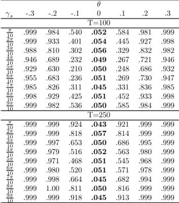
In the …rst experiment we consider a simple pure cyclical model, (1 2 cos _sL+L²)^d+ x_t ="_t

in order to analyze the empirical size and power of ⁽¹⁾_W, asymptotically distributed as ²₍₁₎, when testing H0 :d= 1 with true values given by d= 1 and in[ 0:3;0:3]:We consider 5000 replications and "_t iidN (0;1). Since the Gegenbauer frequency _s is a ‘free’parameter, we set _s = s =10; with s = 1; :::;9. The rejection frequencies for a nominal signi…cance level of 5% and sample sizes of T = 100 and T = 250are shown in Table 1.

The test shows approximately correct size and good power performance even in small samples. Only minor di¤erences, following no particular pattern, arise across the frequencies s

considered. For non-zero vales of ; we observe several interesting features in the empirical power functions. First, given s and T, power tends to exhibit a symmetric U-shape …gure around the =2 frequency, which is more evident for small values of j j: This suggest that, the larger the di¤erence j s =2j with _s 2 (0; ); the more powerful the testing procedure becomes. The dependence of power on the particular frequency the test is related to is not sur- prising, since the variance of the regressor (and hence, the signal-to-noise ratio and, eventually, the power of the test) depends on the speci…c frequency, ; considered and, more generally, on ; see Appendix A for further technical details. Furthermore, if we compare these results to those in Breitung and Hassler (2002, Table 1, p.176) for the zero-frequency case, the power observed at the long-run frequency is approximately of the same order as that for = =2:

This suggest that, everything else equal, fractionally-integrated dynamics are generally easier detected at the cyclical than at the zero-frequency. A similar feature appears when dealing with = (not reported here) for which power is similar to that of = =2.² Dealing with the non-zero frequency also has other bene…ts in terms of power. For …xedT and _s, the power functions tend to be symmetric around = 0, since only the size of 0; and not its sign,

1The dataset in Bouette et al. (2006), refering to hourly average wind speeds measured between 1951 and 2003, includes over 16,000 observations. Soares and Souza (2006) consider two years of hourly electricity demand.

Gil-Alana (2005) studies US monthly in‡ation in a dateset with more than 1000 observations.

2Note that the asymptotic variance is proportional to ( );see Appendix A. This is a positive, symmetric and non-continuous function on[0; ]that takes minimum value ( ) = ²=6for =f0; =2; g;and maximum value given by lim _!₀ ( ) =lim _! ⁺ ( ) = 2 ²=3: We therefore can expect a discontinuity in the power function for the case = 0 + or = even for an arbitrarily small >0:

(18)

seems to drive the probability of rejection. This does not seem to be the case for the zero- frequency case analyzed in Breitung and Hassler (2002), where the LM test is likely to reject more easily if < 0. Finally, power is largely enhanced even for a small sample of T = 250;

and virtually reaches 100% for all the tests whenT = 500, thus showing the consistency of the testing procedure even in small samples.

Second, we consider a more general two-factor cyclic model given by, (1 2 cos ₁L+L²)^d¹⁺ ¹(1 2 cos ₂L+L²)^d²⁺ ²x_t ="_t:

We want to address the ability of the unrestricted joint test ⁽²⁾_W;distributed asymptotically as

2

(2), as well as the joint restricted test ⁽²⁾ discussed in Corollary 4.2, and individual squared t-tests, say ⁽¹⁾₁ and ⁽¹⁾₂, distributed asymptotically as ²₍₁₎; to detect fractionally-integrated dynamics. Subset-testing is discussed in Corollary 4.1. As before, we setd₁ =d₂ = 1;and 1; ₂ in[ 0:3;0:3];considering5000replications and"_t iidN(0;1). The joint test ⁽²⁾_W is expected to reject the null hypothesis if fractional integration is present in, at least, one of the frequencies involved, while the individual tests may only reject when fractional integration occurs at the frequency they are related to. The restricted joint test ⁽²⁾ should be more e¢ cient than ⁽²⁾_W when the restriction ₁ = ₂ is true, but it is expected to exhibit less comparative power to reject the false null otherwise.

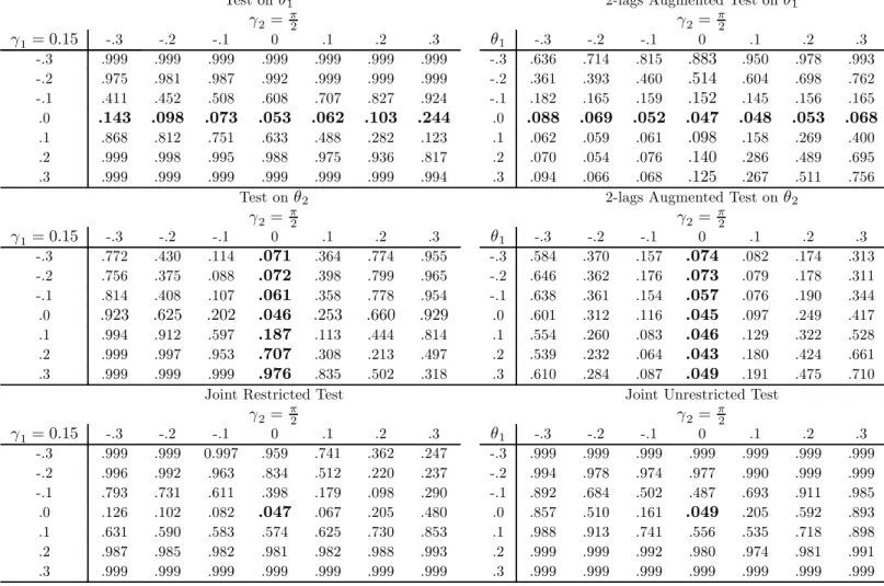
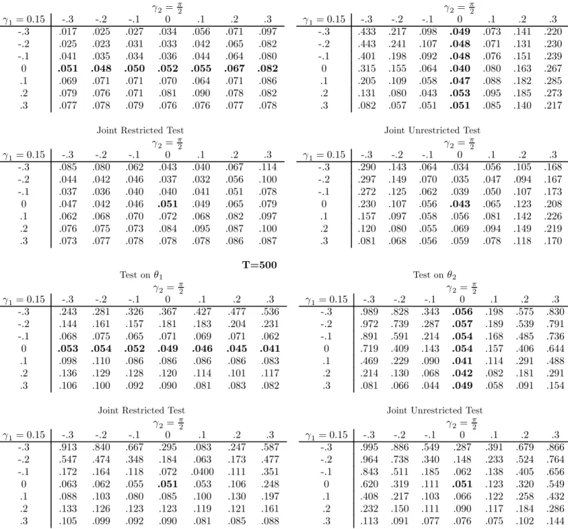
In view of the previous experiment, we expect the power function to depend on the value of = ( ₁; ₂)⁰: We set ₁ = 0:15 =20; corresponding to the estimated frequency of the business cycle by the NBER, and consider what seems to be the most unfavorable frequency for the tests when dealing with frequencies in(0; ), given by ₂ = =2;which also corresponds to one of the harmonics of quarterly and monthly seasonality. For frequencies 2 (0; ) away from =2, further simulations (not reported here) showed a much better statistical performance both in terms of size and power. The rejection frequencies for a nominal signi…cance level of 5% and sample length T = 100 are shown in Table 2.

Several interesting features emerge from this experiment. First, we comment the results for the individual tests ⁽¹⁾_0:15 and ⁽¹⁾₌₂. When d₁ = 1; and d₂ = 1 + ₂; both tests have approximately correct size when 2 is close to zero. However, when j ²j moves away from the origin, ⁽¹⁾_0:15 may show size departures with respect to the nominal size, which are particularly important when 2 > 0: This is also true for the ⁽¹⁾₌₂ test when d₂ = 1 and d₁ = 1 + ₁; now noting massive size distortions for large 1 >0: As remarked in Section 4, these distortions are originated from residual autocorrelation resulting from misspeci…cation. For moderate degrees of autocorrelation, size departures can be considerably reduced by augmenting the auxiliary regression with p lags of the dependent variable. Table 1 shows, forp = 2, that augmentation is e¤ective in reducing the distortion, particularly in the region > 0 in which the e¤ect was more pronounced. However, as usual, empirical size is corrected at the cost of power reductions, which in this context can be large for the alternatives > 0: Finally, it is interesting to note that, when the empirical size approaches the asymptotic nominal level (correct speci…cation), the power of the ⁽¹⁾₌₂ test is only slightly smaller than that observed when the DGP only includes a Gegenbauer polynomial. Similar behavior can be observed for ⁽¹⁾_0:15.

In relation to the joint test statistics ⁽²⁾ and ⁽²⁾_W; we observe that the restricted test is more powerful than the latter when the restriction 1 = ₂ is true, but it is also considerably

(19)

less e¢ cient in the general context 1 6= ₂, particularly for small values of j j: Both tests tend to reject more easily the (false) null when fractional integration is present at the frequency0:15;

i.e., at the frequency for which the magnitude j ^s =2j is larger. For instance, ifd₁ = 1 0:1 and d2 = 1; the power of ⁽²⁾ and ⁽²⁾_W is, approximately, 39.8% and 48.7%, respectively. In contrast, ford₁ = 1 and d₂ = 1 0:1;the power is only 8.2% and 16.1%. When both 1 and 2

move away from the origin, the power of joint tests, particularly that of ⁽²⁾_W;largely increases.

We note that the power of ⁽²⁾_W seems to be symmetric for the set of frequencies considered, whereas ⁽²⁾ tends to reject more easily when 1 >0and 2 <0 than in the converse case. For instance, the power of ⁽²⁾ for 1 = 0:3and 2 = 0:3is almost 100%, whereas it is around 25%

for 1 = 0:3 and 2 = 0:3: By sharp contrast, the power of the unrestricted test ⁽²⁾_W in any of these cases is almost 100%. Finally, and as in the case of the one-factor model, considering larger samples, T =f250;500g;leads to considerable improvement of the statistical properties of all the tests. We do not present these results to save space, but these are available upon request.

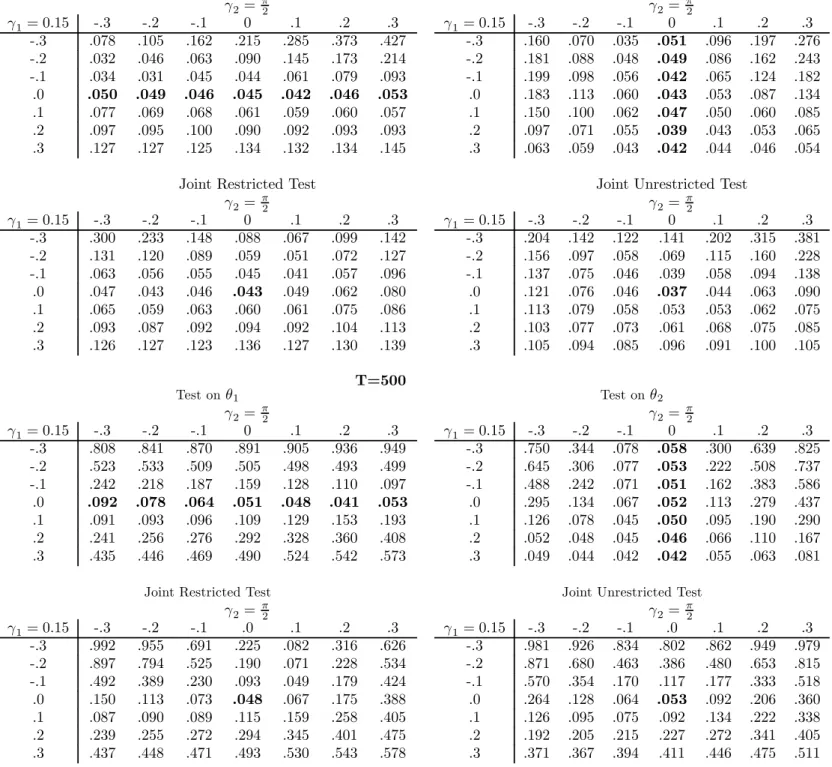
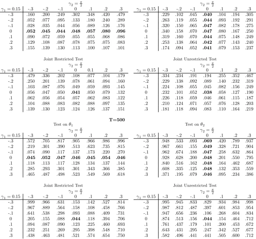
Finally, the last set of experiments considers again the two-factor …lter (L; ) = (1 2 cos ₁L+L²)^d¹⁺ ¹(1 2 cos ₂L+L²)^d²⁺ ² now allowing for stationary and invertible ARMA patterns in the error term, i.e., we analyze the performance of the augmented-based test statistics when the DGP is,

(L; )xt = "t

(1 aL)"_t = (1 bL)v_t;

under the restriction jaj < 1 and jbj < 1. We …rst focus on ARMA(1,1) dynamics and, as in Demetrescu et al: (2007), set a = 0:5 and b = 0:5: The ARMA(1,1) model is particularly relevant because short-run dynamics in empirical applications are usually characterized par- simoniously through this speci…cation. Additionally, we analyze in more detail the e¤ects of persistence through an AR(1) with parametera=f0:5;0:75;0:9g and b= 0 in the above spec- i…cation. Since for empirical purposes the underlying structure of the short-run component is typically unknown, we explore the e¤ects on the tests when the number of lags to be included in the auxiliary regression are determined according to Schwert’s rule, p= 4(T =100)¹⁼⁴ , as this showed the best performance in the empirical analysis in Demetrescuet al: (2007). The rejection frequencies for the individual and joint tests given ARMA(1,1) patterns forT =f100;500g are shown in Table 3, whereas Tables 4 and 5 report the respective empirical results for the AR(1) errors given the values of the autoregressive coe¢ cient a.

We …rst comment the results for the ARMA(1,1) dynamics. The general conclusions that arise for the weakly-dependent case are similar to those observed for the i.i.d case, although we observe several quantitative changes. Augmentation proves able to help correct the empirical size for all tests, and only small undersizing e¤ects are observed in our simulations. However, and as shown in previous literature, ensuring correct empirical size against general ARMA dynamics through augmentation in small samples, such asT = 100, comes usually at the cost of potentially large reductions in power in relation to the i.i.d. case. This pervasive e¤ect has been widely documented in the unit-root literature, where the augmented Dickey-Fuller regression is probably the most widely used in applied settings. In fact, the power of the individual and the joint tests shows …gures similar in magnitude to those observed in Demetrescuet al: (2007) for the fractional unit root case. By sharp contrast to the unit-root case, fortunately, power