Towards efficient audio-visual source separation and synthesis

Towards Efficient Audio-Visual Source Separation and Synthesis

Juan Felipe Montesinos

TESI DOCTORAL UPF / year 2023

THESIS SUPERVISOR

Gloria Haro

Department Department of Information and

Communications Technologies

Insights and acknowledgments

I would like to start talking about “the PhD”. Before starting it, I though doing a PhD was about being a smart guy with clever ideas. Then, I realized it has many more dimensions and factors. The success is not only about you, but maybe, about having good reviewers, or computatio- nal resources. Maybe it is about having the right people around, or having an idea in the right moment. Funny fact, deep learning (backpropagation to be technical), the technology called to change the present and the futu- re, was invented in the 60s. The success could be a matter of appearing in the queue of Arxiv, or being cited in a tweet or a paper. In short, the PhD, for better or worse, is a whole environment with many dimensions interlaced.

I really believe, despite I’m very rational, that life guides us. I met my PhD supervisor, Gloria Haro, back in 2017, while carrying out my MSc.

in computer vision. She was teaching 3D vision and she was conside- red as great teacher among us, the students. By the end of my masters, I was supposed to travel to Paris to carry out my master thesis in a well- positioned company. The day before flying, I was told the university and the company couldn’t reach and agreement, my final project was cance- led. That was a tough moment, I was disoriented but, as I mentioned, life guides us. Gloria offered me to carry out the master thesis with her, which led to this PhD afterward. From my point of view, Gloria has be- en a wonderful supervisor, she is very supportive and understanding, and works tirelessly. Truly a role model. My master thesis was supervised as well by a PhD student, Olga Slizovskaia, who later became my collea- gue. Same as Venkatesh Kadandale, another good colleague whom I met by the beginning of the PhD. Despite the insightful research talks we may have had, I really appreciate having someone who understands the very specific frustration that audio-visual field and ML entails. Sometimes we forget mental health is a thing. Likewise, I cannot forget to mention Patri- cia Vitoria and Adri`a Arbu´es who always were up for a coffee or bringing funny moments that made the lab to be alive. I’m also grateful to have had the opportunity to collaborate with Daniel Michelsanti at Oticon, in Denmark. Everyone at Oticon were very friendly, which made it a great

experience.

This thesis was very conditioned by the COVID pandemic. Virtual conferences couldn’t recreate the human perspective of on-site conferen- ces: discovering new cultures and countries, networking, meeting new different people that may give you support, insights, opinions or new points of view about topics one would never wonder. However, facing such hard times helped me to learn about myself and probably changed my life, my mindset, and my way of seeing the world.

Lastly, taking a look back at my childhood, I feel I need to dedicate a small honorific mention to my mother, Pilar Garcia. She raised me and supported me, following the idea that education is the best gift a person can be given.

That being said, I find the PhD has been a great experience. No mat- ter how successful or not it can be considered by society, it is now an important part of who I am, and I wouldn’t change that.

Abstract

Our brain has the innate capability of isolating different sounds in noisy environments (the cocktail party problem), as well as understanding the relationship between what we see and what we hear. This thesis aims to bring these human cognitive skills to computers by contributing to the im- provement of speech, singing voice and music sound source separation as well as speech inpainting. To do so, we explore new video representations and their suitability for the aforementioned tasks. In case of audio-visual voice separation, we used face landmarks, which encode motion and drop appearance. This allows developing lightweight, real-time audiovisual sound source separation systems. We show how visual information can be beneficial in noisy or multivoice environments, and we propose a deep neural network competitive to state-of-the-art models that exploit both, motion and appearance.

Speech inpainting can be seen as an extreme case, when the accompa- niment sources are so noisy that no signal can be recovered or the speech signal is corrupted. We show how deep-learning-based visual embeddings extracted from large-scale models encode enough information to recon- struct long gaps of speech, up to 1.6s. We also show how the audio-visual models do outperform audio-only systems.

Resumen

Nuestro cerebro tiene la habilidad innata de aislar diferentes sonidos en ambientes ruidosos (Efecto de fiesta de c´octel), as´ı como de entender la relaci´on entre aquello que vemos y o´ımos. Esta tesis tiene como objeti- vo trasladar estas habilidades cognitivas, caracter´ısticas de los humanos, a los ordenadores. De esta forma, se busca contribuir a la mejora de, por un lado, la separaci´on de sonidos tanto en el ´ambito de los discur- sos hablados, como en el de la m´usica y la voz cantada; y por otro a la reconstrucci´on contextual de discursos hablados. En el caso de la sepa- raci´on de discursos hablados, usamos marcadores faciales que codifican el movimiento y dejando de lado la apariencia. Esto permite desarrollar sistemas audiovisuales de separaci´on de sonidos en tiempo real y ligeros.

Asimismo, mostramos como la informacion visual puede ser beneficiosa en entornos ruidosos o con m´ultiples voces, y proponemos una red neural competitiva con modelos del estado del arte que utilizan movimiento y apariencia.

La reconstrucci´on del discurso hablado puede ser visto como un caso extremo, cuando las fuentas que acompa˜nan al discurso son tan ruidosas que este no se puede recuperar, o cuando la propia se˜nal est´a corrupta.

En este escenario mostramos como representaciones de la informaci´on visual extra´ıdas con modelos de gran tama˜no codifican suficiente infor- maci´on para reconstruir largos segmentos de discurso hablado, de hasta 1.6s. Tambi´en mostramos como los modelos audiovisuales superan a los modelos que s´olo utilizan audio.

Contents

List of figures xiii

List of tables xvii

List of abbreviations xvii

1 INTRODUCTION 1

1.1 Motivation . . . 2

1.2 Audio-Visual in Machine Learning: Introduction and Chal- lenges . . . 6

1.2.1 Introduction to Multimodal Analysis . . . 6

1.2.2 Challenges . . . 7

The curse of multimodal . . . 7

Computational cost . . . 8

Storage Cost . . . 9

Data Curation, Data shortage and Data Quality . 10 Reproducibility . . . 11

Ethics and data privacy . . . 12

1.3 Thesis Scope and Contributions . . . 13

1.4 Outline of the thesis . . . 15

2 THEORETICAL BACKGROUND 17 2.1 Audio representations . . . 18

2.1.1 Waveforms . . . 18

2.1.2 Time-frequency representations: Short-time Fourier

Transform . . . 18

2.1.3 The Human Auditory System and Mel Spectrogram 20 2.2 Deep neural networks . . . 23

2.2.1 The U-Net . . . 23

2.2.2 Transformers . . . 24

2.3 Visual representations . . . 26

2.3.1 Motion, graphs, and face landmarks . . . 26

2.3.2 Audio-visual HuBERT . . . 27

2.4 Foundations on Sound Source separation . . . 28

2.4.1 Problem formulation . . . 28

2.4.2 Sound Source Separation in the time-frequency domain . . . 30

2.4.3 Sound Source Separation in the time domain and hybrid approaches . . . 32

2.4.4 Sound Source Separation before Deep Learning . 33 2.4.5 Mix-and-separate Strategy . . . 33

I Audio-visual Source Separation 35

3.2 Related Work . . . 39

3.3 Dataset . . . 42

3.3.1 OpenPose Skeletons . . . 42

3.3.2 Timestamps estimation and skeleton refinement . 44 3.4 Experiments . . . 45

3.4.1 Architectures and training details . . . 45

3.4.2 Data pre-processing . . . 48

3.4.3 Mix-and-separate . . . 48

3.4.4 Results . . . 49

3.5 Conclusions . . . 50

4 CNN-BASED SINGING VOICE SEPARATION 51

4.1 Introduction . . . 52

4.2 Related work . . . 54

4.3 The Dataset . . . 55

4.4 Singing voice separation model . . . 57

4.4.1 Pre-processing . . . 61

4.4.2 Training strategy, training target and loss . . . . 61

4.5 Experiments . . . 63

4.6 Conclusions . . . 69

5 TRANSFORMER-BASED SPEECH AND SINGING VOICE SEPARATION 71 5.1 Introduction . . . 72

5.2 Related work . . . 74

5.3 Approach . . . 76

5.3.1 The AV Voice Separation Network . . . 76

5.3.2 Low-latency data pre-processing . . . 81

5.4 Datasets . . . 83

5.5 Experiments . . . 84

5.5.1 Audio-visual transformer . . . 85

5.5.2 Speech separation . . . 86

5.5.3 Singing voice separation . . . 92

5.6 Conclusions and Future work . . . 93

II Audio-visual Inpainting 95

6.2 Approach . . . 99

6.2.1 Signal Model . . . 99

6.2.2 Proposed Framework . . . 99

6.3 Experiments . . . 102

6.3.1 Audio-Only and Audio-Visual Baselines . . . 102

6.3.2 The Dataset . . . 102

6.3.3 Loss, Data Pre-Processing and Model Setup . . . 103

6.4 Results . . . 104

6.4.1 Performance Measures . . . 104

6.4.2 General Performance . . . 105

6.4.3 Performance vs Segment Duration . . . 105

6.5 Conclusions and Future Work . . . 107

7 CONCLUSIONS 109 7.1 Overview . . . 109

7.2 Limitations and future work . . . 111

7.3 List of contributions . . . 112

In-proceedings publications . . . 112

Workshop contributions . . . 113

Datasets . . . 114

List of Figures

2.1 Time representations of a periodic sound wave. Illustra- tion from [Kiper, 2016]. . . 18 2.2 a) Speech waveform and b) its corresponding spectro-

gram. Illustration from [Lu et al., 2018]. . . 20 2.3 Mel scale. Illustration from [Appleton et al., 1975]. The

Mel scale’s analytical expression is2595 log₁₀(1+f /700), wheref is frequency (Hz). . . 21 2.4 Mel filterbank (23 filters) as a function of STFT with DFT

size 128. Illustration from [Benesty et al., 2008]. . . 22 2.5 Original U-Net architecture [Ronneberger et al., 2015]. . 23 2.6 Example of landmarks extracted from a high-quality video

with large head displacements and broad points of view at 1 FPS. Frames correspond to Anne Hathaway’s speech:

Paid Family Leave. . . 26 2.7 Energy distribution of a speech sample along frequency

and time. Note that the energy distribution along fre- quency is log-scaled. . . 31 3.1 Solos and URMP instrument categories. Image adapted

from [Li et al., 2019]. . . 42

3.2 Considered architectures. Left, Sound of Pixels: The net- work takes as input a mixture spectrogram and returns a binary mask given the visual feature vector of the de- sired source. Right, Multi-Head U-Net: It takes as input a mixture spectrogram and returns 13 ratio masks, one per decoder. . . 46 4.1 Acappelladataset statistics. . . 57 4.2 Y-Net model scheme. The system works with chunks of

4n seconds, where n ∈ N. The audio network takes as input a256 ×16T n complex spectrogram and returns a complex mask. The visual network in case of Y-Net-m and Y-Net-mr, is the video network (in red), which takes as input a set of 100nframes cropped around the mouth of the target singer. In case of Y-Net-g and Y-Net-gr, the vi- sual network is the graph network (in green) which takes as input a sequence of 68n landmarks of the face of the target singer. The visual features are fused with the au- dio network’s latent space through a FiLM layer (we use T = 16). The FiLM broadcasts the 256×1×T visual features into the 256×16×T audio ones. The spatial blocks of the U-Net downsample in both, the frequency and the temporal dimension, while the frequential block downsamples along the frequency dimension only. . . . 59 4.3 Results in the unseen-unheard test set: left, one lead voice

setup; right, two lead voices setup. Different symbols are assigned to the different models and different colours to the different volume levels of the target voice. . . 67 5.1 Audio-visual voice separation network. Audio and video

features are concatenated in the channel dimension before being fed to the transformer. . . 77

5.2 Frame example fromVoxceleb2[Chung et al., 2018] with partial occlusions. Thanks to the landmark estimation together with the registration we can estimate the unoc- cluded lips. . . 83 5.3 Three proposed ways to feed a transformer with an audio-

visual signal. Left: audio-visual signal, middle: video to the encoder and audio mixture to the decoder, right:

audio-visual signal to the encoder and clean audio to the decoder. . . 85 5.4 Scatter plot showing the difference in SDR and SIR,∆SDR

and∆SIR, as functions of the SDR and SIR of the input mixture in the unseen-unheard wild and clean test sets.

The difference is:∆SDR =SDR(VoViT)−SDR(Visual Voice) so a positive value means VoViT outperforms Visual Voice. 89 6.1 Proposed audio-visual model. The pre-trained video en-

coder corresponds to [Shi et al., 2022]. . . 100 6.2 Comparison of performance vs corruption duration eval-

uated in the test set (see Sec. 6.3.2). . . 104 6.3 Sentencelwib4afor speaker 34 in the test set. Transcrip-

tion: ”lay white in b four again”. The region within the green square indicates the corrupted area. In practice that region is set to zero as input to the network. . . 106

List of Tables

1.1 Number of training parameters in millions (M) for VGG, ResNet and DenseNet models [Leong et al., 2020]. . . . 9 2.1 Most common standards in video for 17:9 and 16:9 for-

mats and the storage cost of a single frame. The typical resolution of speaking face is based on a single speaker giving a speech from a tribune. We refer to Anne Hath- away’s speech: Paid Family Leave as an example. The video can be found athttps://www.youtube.com/

watch?v=gkr57P0fwbI . . . 27 3.1 Statistics of Solos Dataset . . . 43 3.2 Benchmark results. SoP original weights, SoP-Solos: Sound

of Pixels trained from scratch on Solos. SoP-ft: Sound of Pixels finetuned on Solos. MHU-Net: Multi-head U-Net with 13 decoders. . . 50 4.1 Number of parameters (M for million) for the different

architectures compared to common networks in computer vision (ResNet18 and 3D-ResNet18). . . 60 4.2 Ablation study on the unseen-unheard test set in the two

lead voices setup. . . 64 4.3 SDR results in the two lead voices setup for different

methods across languages, both in seen-heard and unseen- unheard test sets. SDR results also for the multi-voice case. LLCP stands for the work at [Ephrat et al., 2018]. . 65

4.4 Comparing singing voice separation performance based on gender, in the two lead voices setup in the unseen- unheard test sets. The values are in SDR. . . 68 4.5 Ablation study on the percentage of mixtures contain-

ing two lead voices in the training of the Y-Net-gr model (note that 0% corresponds to the Y-Net-g model). Results on the unseen-unheard test set. . . 69 5.1 Ablation study: performance of different ways of feeding

a transformer with an audio-visual signal and comparison to Y-Net model [Montesinos et al., 2021]. Evaluated in Acappella’sunseen-unheard test set. Y-Net metrics taken from Acappella. In this table N = 4 (the number of blocks in the transformers) in order to adapt the number of parameters to the size ofAcappelladataset. . . 86 5.2 Ablation of different variants of the refinement stage and

number of blocks in the transformer of the first stage.

VoViT-s1 stands for the model with just the first stage, r stands for the number of recurrent passes in stage 2. For the stage 2 we considerered both, the Visual Voice’s UNet (VV) [Gao and Grauman, 2021] and the Y-Net’s UNet (YN) [Montesinos et al., 2021]. . . 88 5.3 Evaluation onVoxceleb2unheard-unseen test sets (mean

±standard deviation). VoViT stands for our model with the 10-block AV ST-Transformer with the Y-Net’s UNet backbone as the lead voice enhancer. Number of param- eters in millions. Results in the first block are taken from the original papers. . . 90 5.4 Latency estimation for the different variants of VoViT.

Average of 10 runs, batch size 100. Device: Nvidia RTX 3090. GPU utilization>98%, memory on demand. Two forward passed done to warm up. Timing corresponds to ms to process 10s of audio. . . 91

5.5 Singing voice separation. Mixtures of two singers with no additional accompaniment from the test set unseen- unheard (only samples in English) ofAcappella. Results in top block: models trained directly with samples of singing voice; bottom block: models trained with speech samples. . . 92 6.1 Performance scores averaged across test set. Corrupted

segment lenghts sampled from a uniform distribution. . . 105

List of abbreviations

AO Audio Only. 98 AV Audio-Visual. 2

AVSI Audio-Visual Speech Inpainting. 7 AVSS Audio-Visual Source Separation. 7

BERT Bidirectional Encoder Representations from Transformers. 28 BSS Blind Source Separation. 28

CASA Computational Auditory Scene Analysis. 33 CNN Convolutional Neural Network. 8

DFT Discrete Fourier Transform. 19 ELU Exponential Linear Unit. 103 FiLM Feature-wise Linear Modulation. 8 GCN Graph Convolutional Network. 27 GELU Gaussian Error Linear Unit. 79 ICA Independent Component Analysis. 33

LR Learning Rate. 47

MAE Mean Absolute Error. 103 MHU-Net Multi-head U-Net. 45 MIR Music Information Retrieval. 38 ML Machine Learning. 4

MLP Multi-Layer Perceptron. 100 NLP Natural Language Processing. 6

NMF Non-negative Matrix Factorization. 33 NN Neural Network. 6, 7

PLCA Probabilistic Latent Component Analysis. 33 RNN Recurrent Neural Network. 78

ROI Region of Interes. 10

SAR Sources to Artifacts Ratio. 49 SDD Solid State Drive. 9

SDR Source to Distortion Ratio. 49 SIR Source to Interferences Ratio. 49 SoP Sound of Pixels. 45

SOTA State of the Art. 14

ST-GCN Spatio-Temporal Graph Convolutional Network. 14 STFT Short-Time Fourier Transform. 19

URMP University of Rochester Multi-Modal Music Performance Dataset.

39, 110

Chapter 1

INTRODUCTION

1.1 Motivation

Once Rene Descartes wondered if the world was real or just an illusion created by an evil genius. Likewise, we would like to reflect on how do we perceive the world.

Most events that take place in our world generate a rich source of visual and auditory signals. Imagine having dinner in a cozy table with friends and family. All of a sudden, a bottle falls onto the floor in the other side of the table. If we just use the sight, we cannot know whether the bottle has broken or not, since the table occludes the event, or even what the bottle is made of. If we just use the hearing, we can perceive whether a piece of glass or plastic has broken or fallen, but we would not be able to identify which object was it.

Acoustic and visual signals are two counterparts from the same event in the real word. That is why, our perception is highly multimodal. Audio- visual (AV) signals can help to disentangle ambiguities: distinguishing between a dog or a wolf, whether a cup is made of glass or plastic or to track and localize better [Charbonneau et al., 2013, Hofman et al., 1998].

There are even more constrained cases, e.g., to infer the distance of a thunder, we need both the visuals and the acoustics of the event. These examples aim to illustrate how acoustic and visual signals are often com- plementary and can improve our perception. It is not surprising that the human cognitive system evolved to learn efficiently from multisensory stimuli [Shams and Seitz, 2008].

Among all natural phenomena, speech is one of the most relevant ones for humans. We are constantly exposed to speech on the TV, on social net- works, at work, at home... Speech is so important that, through evolution, humans developed special areas in the brain devoted to the production and comprehension of natural language [Dronkers and Ogar, 2004]. Un- surprisingly, speech is not processed as an acoustic signal by the brain, but as an audio-visual one. In [Chen, 2001] the authors show how certain phonemes (the smallest phonetic unit in a language that is capable of con- veying a distinction in meaning) that are hard to distinguish acoustically can be distinguished audiovisually. In [Fisher, 1968] the authors illustrate

how, for a given phoneme, the perceived sound can change depending on the visuals from the lips.

We can trace the origins of speech back to singing voice, which is related to the origin of the voice. The most accepted theory is speech appeared as an evolution from singing voice, understood as the “vocal- ization” to express emotion and imitate natural sounds, as explained in [Aiello and Dunbar, 1993, Jespersen, 2013]. Even though both, singing voice and speech share some characteristics, e.g., intelligibility, they are substantially different. Whereas speech aims to transmit information and certain emotions (anger, sadness, happiness...), singing voice also includes melody and rhythm, pursuing aesthetical sounds in addition to content.

For this reason, singing voice is often ornamented with resources such us vibrato or humming, originating a great amount of sustained vowels and notes.

Singing voice is intimately tied to music. Music shares its origin with singing voice, and both have played an important role in our evolution [Schulkin and Raglan, 2014]. That may be the reason voice is considered as the original instrument. At first look, we may think of music as uni- modal event, however, there are studies showing that the nature of music perception is multimodal [Leman, 2017, Thompson et al., 2005]. Music is an AV performance, and it is intrinsically related to dance. Worldwide, folkloric music and tribal songs are usually paired to different dances.

Even in our days, all the modern songs are usually released as video clips, not just audio clips. And many live performances involve visuals: instru- mental concerts, ballet, music concerts, films... In fact, we prefer AV performances over audio-only ones. [Platz and Kopiez, 2012] concludes we score higher AV performances in terms of overall impression, expres- siveness, likability or quality.

Due to the aforementioned reasons, we have spent decades develop- ing systems which can capture these audio-visual streams as we perceive them, with the highest fidelity. With the democratization of these devices and the expansion of internet, billions of hours of recordings and gener- ated content are available in public platforms such as YouTube, Twitch, Vimeo, Instragram... Unfortunately, proper systems to exploit all this in-

formation were not developed in parallel due to lack of computational power and effective techniques. More recently, with the rise of machine learning (ML), researchers and companies started developing effective and automatized tools to make profit from all this data. Initially, ML was focused on supervised learning. Supervised learning algorithms assume access to human-labeled datasets to train ML models. This scenario was feasible for computer vision algorithms involving images, as humans can understand images without any training; but it is prohibitively expensive for video, where the amount of information to be labeled is huge. It is also unfeasible for audio, where, unlike images, humans are cannot inter- pret their representations (waveforms, spectrograms etcetera...) without training and expertise.

In order to process these millions of hours of video, other kinds of algorithms that do not require fully supervision, i.e., human-labeled data, must be developed. Inspired by how humans can learn autonomously, this thesis aims to find different ways of learning from audio-visual content and the natural correlation between audio and video to train deep learning algorithms with few or no human-labeled data. More specifically, this thesis contributes with new self-supervised audio-visual deep-learning- based models for speech inpainting and for source separation in different contexts: musical instruments, singing voice and speech.

AV speech comprehension, separation, and enhancement play an im- portant role. AV Voice separation can help in speaker diarization and transcription. For example, in talk shows where several people speak at the same time. Or in parliamentary sessions, it would be possible to track each speaker’s speech, obtaining clean isolated recordings and transcrib- ing them. The same applies to a news broadcast from the street, or for multilanguage doubling of speeches, where the journalist’s voice could be enhanced for viewer’s convenience. In conferencing systems, back- ground noises or leaking voices which do not correspond to the speaker can be removed. In the worst case, for applications where audio is totally unusable, speech reconstruction from lips can substitute this enhance- ment/separation process.

Regarding music and singing voice, isolating different instruments or

voices can be beneficial for transcription and educational purposes. It could also be applied in the context of remixing, where each source can be isolated, and the composition can be resynthesized with different filtering, tempo, or sources.

1.2 Audio-Visual in Machine Learning: Intro- duction and Challenges

1.2.1 Introduction to Multimodal Analysis

As mentioned in Sec. 1.1, AV music and voice separation, as well as AV speech inpainting can be tackled with self-supervised algorithms.

The goal of self-supervised techniques is to train ML algorithms with- out any human-annotated data. In unimodal domains, e.g., vision, nat- ural language or audio, a typical procedure is reconstructing, partially or totally, the input data. Autoencoders are a good example of self- supervision [Bank et al., 2020, Cinelli et al., 2021], where a neural net- work (NN) maps the input data to a low-dimensional space (compres- sion) for then reconstructing it (decompression). Or inpainting, which is a traditional self-supervised task in vision, where an image is masked partially to infill the masked content coherently with the rest of the im- age. Transformers [Vaswani et al., 2017] are one of the most powerful architectures to process sequences. They can make profit frommask-and- reconstructschedules in several fields such us Natural Language Process- ing (NLP), audio, or AV [Devlin et al., 2018, Hsu et al., 2021], improving performance, generalization, and robustness. This idea will be detailed in Sec. 2.2.2.

In a multimodal scenario, possibilities beyond self-reconstruction ap- pear. The key idea is to exploit the relationship among modalities as a supervision cue. In the AV field, these are the correspondences between audio and video in recordings. A good example is cross-modal estima- tion, where the goal is to infer audio from video or the other way around, e.g., lip-to-speech estimation [Mira et al., 2022], or the aforementioned mask-and-reconstructpre-training technique [Shi et al., 2022]. Similarly, cross-modal correspondence aims to solve whether an audio and video streams match or not [Arandjelovi´c and Zisserman, 2018]. If audio and video streams are finely correlated, AV synchronization can be estimated [Kadandale et al., 2022, Truong et al., 2021, Chen et al., 2021]. Other in- teresting tasks which involve correspondence are cross-modal style trans-

fer [Li et al., 2022] or zero-shot learning [Mercea et al., 2022], where au- dio, video, and text are mapped into a common latent space.

Lastly, it is worth mentioning some important multimodal tasks, though these are fully supervised: text-to-speech [Hsu et al., 2021], or AV speech recognition [Shi et al., 2022].

In the context of this thesis, there are works addressing AV music source separation, such as [Zhu and Rahtu, 2020], or speech separation [Gao and Grauman, 2021] among others. However, AV singing voice separation was not explored in the literature before. AV speech inpainting (which is similar to lip-reading) was already explored for small datasets in [Morrone et al., 2021]. A detailed literature review of both, AV source separation (AVSS) and AV speech inpainting (AVSI) is carried out in Secs. 4.2 and 5.2; and Sec. 6.1 respectively.

Despite the rich variety of tasks to solve, there are certain challenges that motivated and constrained the scope of this thesis. In the next section, we will describe them.

1.2.2 Challenges

The curse of multimodal

A really common problem in multimodal tasks is that one modality tends to dominate over the other [Michelsanti et al., 2021, Wang et al., 2020].

For example, in the AV speech recognition task, where the goal is to tran- scribe AV speech recordings, audio is often enough to solve the task, and it is the most related modality to text. Learning to extract meaningful information from the visuals is slower than learning from audio, thus, visuals are ignored. This has led to different ways to fuse AV informa- tion, often inspired by biology; and strategies to force NN models to at- tend both modalities. Regarding the fusion stage, we can classify existing strategies into:

• Early fusion,where the acoustic and visual modalities are concate- nated as raw or roughly raw data (e.g. [Morrone et al., 2021]).

• Mid fusion,where the acoustic and visual modalities are first pro- cessed independently for later on being fused and processed jointly (e.g. [Owens and Efros, 2018]).

• Late fusion,where the acoustic and visual features are processed separately and the information is shared via metric learning (e.g.

[Korbar et al., 2018])

Regarding the fusion mechanism, there are three main groups: by using attention [Chen et al., 2021], by concatenation [Morrone et al., 2021] or using Feature-wise Linear Modulation (FiLM) [Perez et al., 2018].

Nevertheless, the most effective way depends on training strategies rather than fusion mechanisms. In [Shi et al., 2022], the authors use modal- ity dropout and a mask-and-reconstruct procedure, forcing the network to use the visual modality to accomplish the task. Other strategies can be adding noise to the audio, and the most effective one, posing the problem in such a way that visuals are required to solve the task, as in [Gabbay et al., 2018]. In our case, when working in AVSS, we mix two human voices within the same audio track such that the network must pay attention to motion to figure out the target voice, as we will show in Chapters 4 and 5.

Computational cost

Neural networks suffer to process high-resolution content. 4K (4090 x 2160) and full HD (1920 x 1080) are the standards in video resolution as of today, while NNs usually work with resolutions as small as64×64, 112×112or256×256. Despite some works are starting to close the gap, this is still a big issue in the computer vision community. Calculating coarse numbers for a 25-fps RGB video implies approximately 120 Mbps to process. In case of multimodal information, we require extra 512 kbps corresponding to a 16 kHz audio signal.

There are two common types of NN widespread in image process- ing. 2D convolutional neural networks (CNNs) and transformers. Their extension to video is trivial. In the former case, convolutional kernels

are extended, leading to 3D CNNs. These architectures are data greedy, as there is a big increment in the amount of parameters from 2D CNNs to their 3D counterparts (see Table 1.1), although hybrid solutions ap- peared [Leong et al., 2020, Tran et al., 2018]. In the latter case, no spe-

Model 2D-CNN 3D-CNN

VGG-16 134.7 M 179.1 M

ResNet-18 11.4 M 33.3 M

ResNet-34 21.5 M 63.6 M

ResNet-50 23.9 M 46.4 M

ResNet-101 42.8 M 85.5 M ResNet-152 58.5 M 117.6 M DenseNet-121 7.2 M 11.4 M DenseNet-169 12.8 M 18.8 M

Table 1.1: Number of training parameters in millions (M) for VGG, ResNet and DenseNet models [Leong et al., 2020].

cial adaptations are required. Simply, video can be considered as a longer sequence. This is problematic as transformer’s computational complexity isO(n²)wheren is the sequence length. In any case, the computational cost of both, CNNs and transformers, grows exponentially with the spatial and temporal resolution.

Storage Cost

Besides computational complexity, there is an additional cost that is not usually taken into account. Storage cost. Deep learning requires really optimized pipelines, which often forces using high-end hardware and un- compressed data formats. Working with video often requires long pre- processing pipelines to obtain curated data. A typical pipeline is described in Pipeline 1.

In the hard disk context, Solid State Drive (SDD) disks are a must [Kadve, 2016]. Nowadays, SSD disks’ capacity varies from 128 Gb to 8 Tb, being 1 Tb the most extended size. Giving a glimpse about the

Pipeline 1AV-Dataset Pre-processing

1: Downloading the audio-visual recordings.

2: Video re-encoding (to correct missing frames and have a homogenous frame rate).

3: Audio resampling.

4: Frame-wise detection of the region/s of interest (ROIs).

5: Trimming

6: Cropping around the ROIs.

7: Image alignment (warping).

8: Video resizing.

9: Video compression (if not using raw information)

required storage capacity, one of the standard datasets in the AV speech community,Voxceleb2[Chung et al., 2018], requires more than 1 Tbonce curated. Moreover,Voxceleb2is a +2000-hours low-quality dataset con- formed by YouTube videos. High-quality AV datasets, such as MODAL- ITY dataset [Kawaler and Czy˙zewski, 2019] (≈30h), requires around 213 Gb of hard disk before being curated. In conclusion, working and pre- processing AV datasets is often intractable for many research groups and universities, as this would require specialized knowledge (distributed stor- age and computing...) and lots of storage resources.

Data Curation, Data shortage and Data Quality

A key ingredient to bound computational and storage cost is data curation.

For example, on the TV news, we usually see a presenter in a television studio. If we are analyzing the speech content, e.g., to carry out AV speech recognition, we do not care about the studio but the presenter and, often, just his/her face or mouth. Therefore, the mouth can be considered as the ROI. As shown in Pipeline 1, step 4, we usually find per-frame ROIs, then crop and trim the video to finally align all the frames. This is crucial to reduce the overfitting and both, the storage cost and computational cost (cropped videos are much smaller).

However, this step is not straight-forward in many cases. For human-

related content, there are dozens of algorithms to track the body pose, the hands, or the face, even to extract depth maps or 3D reconstructions. For everything else, the best we can usually find are object detectors. Still, the classes are limited. As a consequence, there is a strong data shortage in many different scenarios. Without robust algorithms, it is not possible to create automatized large-scale datasets from video platforms. Even if it is still possible to gather data manually, in small-scale video datasets (less than 50 hours), a lack of ROIs may lead to overfitting.

Another relevant problem is data quality. Many popular large-scale video datasets have poor quality. This is problematic, as noisy samples are related to the double descent phenomena [Nakkiran et al., 2020]. In small-scale datasets, this noise may prevent NNs from learning useful patterns.

The data issues mentioned in this section affect specially the AV com- munity focused on music analysis. While there are some efforts to in- crease the available data, there is still no suitable large-scale AV mu- sical dataset. To this extent, this thesis contributed to the community with the creation of two different datasets: Acappella dataset, an AV dataset of people singing a cappella [Montesinos et al., 2021]; and So- los , a dataset of musicians solo playing different musical instruments [Montesinos et al., 2020].

Reproducibility

Reproducibility in ML and, concretely, in the AV field, deserves a few words. Despite computers are deterministic, there are several reasons why this is challenging in ML. First, datasets are huge and difficult to track. In an ideal world, we should keep a copy of each dataset once we finish an experiment and process the results. The reality is datasets mutate through time, hence this is unfeasible. That is the case in the AV community, where many datasets are a compilation of YouTube IDs. This provokes further researchers not to have access to exactly the same data, as certain recordings may have been removed. At the time of writing this thesis, one of the most important speech datasets, Voxceleb2 [Chung et al., 2018],

which was available through direct download, was replaced just by the corresponding YouTube links due to copyright issues.

Another remarkable problem is the traceability of the samples. As there are no official training/testing splits, researchers tend to make their own. This process often involves splitting recordings into chunks which are not clearly traced.

Ethics and data privacy

Due to the delicacy of the subject, we will omit any reference in this sec- tion, as the purpose is to reflect certain issues rather than pointing towards specific cases.

Large scale ML models need huge amounts of data. To respond to the growing demand for data, many services, and companies collect user data under abusive terms and conditions with fine print. That is the case for many face swapping services, voice conversion services, smart vehicles equipped with cameras and sensors, coding assistants and a great amount of phone apps including social networks or cloud storage services. A great culprit is the fact many services are cloud based, forcing users to send their personal data, a moment in which they lose any control or track on it.

Another relevant problematic is ML models may exploit data biases and spurious correlations. For example, we can imagine models predict- ing the probability that a person commits a crime based on his appearance.

Or models making use of correlations based on ethnicity in topics such us medical diagnosis, AV tasks involving face or voice synthesis, etcetera...

Lastly, it is worth mentioning generative models are reported to gen- erate training samples and samples with copyright. It is even possible to recover training samples or private information targeting specific samples from trained NNs, as shown in different works in the literature, such as [Haim et al., 2022, Song et al., 2017], or [Wang and Kurz, 2022].

In this thesis, face landmarks and motion embeddings are used in re- placement of raw video, which alleviates the data privacy by dropping the appearance and user identity. This idea will be detailed in Sec. 2.3.1.

1.3 Thesis Scope and Contributions

Once pointed out the problematics of ML and the AV field, let us de- fine the scope of the doctoral thesis. As mentioned in the introduction, this thesis focuses on the development of self-supervised algorithms for processing speech, music and singing voice AV signals. Concerning the above challenges, the goals of the thesis are the following:

1. The design of different NN architectures regarding four pillars: la- tency, performance, self-supervision and real-world applicability.

These architectures involve the following tasks:

(a) Music Source Separation (b) Singing Voice Separation (c) Speech Separation

(d) Audio-Visual speech inpainting

2. The creation of datasets that benefits the AV community and allevi- ates the data shortage, as well as optimal data-loading pipelines to train NNs efficiently.

3. Developing software, libraries, and frameworks which provide tools to work with AV data in a reproducible manner.

This thesis contributed to the development of the audio-visual source separation and audio-visual speech inpainting problems in the following ways, which are sorted historically:

1. AV music source separation: We propose a collection, develop- ment, and preprocessing of an audio-visual dataset of musicians playing solo excerpts based on YouTube videos. We provide Youtube IDs and the corresponding timestamps of relevant segments of each video, body and hand skeletons extracted with an open-source li- brary, Openpose [Cao et al., 2019]. This work was developed in [Montesinos et al., 2020].

2. AV singing voice separation: We address the task of singing voice separation. Due to the lack of public datasets, we collected a 46- hour dataset of a cappella solo singing videos in four languages.

We designed a source separation model that is based on a U-Net ar- chitecture conditioned on motion features. Motion features are ex- tracted with a Spatio-Temporal Graph Convolutional Network (ST- GCN) that receives a sequence of face landmarks as input. We show the superior performance of face landmarks compared to video in small datasets, where overfitting is problematic. Besides, we study the relevance of language in AVSS, showing that NNs can perform similarly for unseen languages. Lastly, we show how audio-visual models for singing voice separation are particularly useful when there are multiple voices in the mixture, or when the volume of the target voice is low compared to the other sources. This work was carried out in [Montesinos et al., 2021].

3. AV speech separation: We develope a new audio-visual architec- ture based on transformers and ST-GCNs that is State of the Art (SOTA) in speech and singing voice separation, showing how land- marks can be competitive against video-based networks on large scale datasets without exploiting appearance attributes. Further- more, we study different transformer variants to efficiently consume audio-visual data. Besides, we propose a two-stage training solv- ing two different optimization problems, which boosts the results in terms of interferences from other sources at a cheap cost. Lastly, we study the suitability of models trained in speech datasets for singing voice, showing a drastic drop in performance, which indicates the necessity of gathering more singing voice data. This exploration was done in [Montesinos et al., 2022a].

4. AV speech inpainting: We propose a state-of-the-art transformer- based architecture that is capable of reconstructing long gaps of corrupted audio by leveraging the visual information. Visual fea- tures are extracted with AV-HuBERT [Shi et al., 2022], which en- code information at a viseme level. We study the degradation of the

generated speech for both AV models and audio-only models. To this extent, we enlarge the gap duration, showing audio-only mod- els collapse while AV models quality is consistent. This work was carried out in [Montesinos et al., 2022b].

1.4 Outline of the thesis

Chapter 1 introduces the reader to the world of multimodal processing in machine learning, briefly revisiting the multimodal perception from a hu- man perspective and its impact on society and evolution as motivation to the problems tackled in the thesis: AV music and voice separation as well as AV speech inpainting. We also overview the challenges in the field, which have constrained the thesis and bounded its scope. The chapter is closed by the thesis’ academic contributions by topics. In Chapter 2, we provide the mathematical and theoretical tooling to understand the acous- tic and visual data representations, the transformations used in this thesis, and foundations on source separation and graphs. Moreover, we explain the main NN’s architectures used, ST-GCNs and transformers.

Afterward, we present two different blocks that cover the main topics of the thesis: the first block, devoted to the AVSS problem and includes Chapters 3-5. Chapter 3 presentsSolos, the dataset of AV music perfor- mances. Chapter 4 presentsAcappelladataset and explores singing voice separation using face landmarks and graphs. Lastly, Chapter 5 addresses AV voice separation using transformers. The second block consists of a single chapter, Chapter 6, which devoted to multimodal speech recon- struction. The thesis ends with a chapter summarizing its content, the conclusions, and proposing future work.

Chapter 2

THEORETICAL

BACKGROUND

2.1 Audio representations

2.1.1 Waveforms

Sound waves are longitudinal mechanical waves that travel through a physical medium, usually air. As longitudinal waves, there exist com- pression and rarefaction stages, where the separation among air particles is larger or smaller than in average. Measuring the pressure allows char- acterizing waves, as shown in Fig. 2.1. These signals were standardized, resulting in different waveform formats [IBM, 1991]. Nowadays, wave- forms are thede factoaudio representation in signal processing.

Figure 2.1: Time representations of a periodic sound wave. Illustration from [Kiper, 2016].

2.1.2 Time-frequency representations: Short-time Fourier Transform

Waveforms are a very low-level representation of sound waves, hardly interpretable by humans. A more intuitive and compact representation of

acoustic information is the time-frequency characterization of waveforms.

In time-frequency characterization, the signal is split into short segments to carry out a frequency analysis on each of them. These representations assume signal properties vary slowly in time, i.e., they are approximately constant within each segment. For example, in case of speech, a phoneme duration is 80 ms in average. Some of the most relevant representations are Constant-Q transform, Wavelet transform, Wigner Distribution Func- tion, Discrete Cosine transform, or Short-time Fourier Transform (STFT).

STFT is specially suitable for source separation, as it is a linear invertible transformation based on the well-known Fourier Transform. That is why, it is widely used in the ML literature and will be the main audio represen- tation in this thesis.

The STFT of a 1D signal can be calculated as a sequence of Fourier Transforms carried out on a windowed signal [Diniz et al., 2010]. Let x(t)be a 1D continuous signal andX(ω, τ)be the corresponding STFT.

Then, STFT can be computed as:

X(ω, τ) = Z ∞

−∞

x(t)g(t−τ)e^−jωtdt

whereg(τ)is the window function.

In practical applications, discrete-time STFT is used. We refer to [Benesty et al., 2008] for detailed information. Assuming nowx(t)is fi- nite, we can define its discrete version, x[t], by sampling the signal at a frequency F_s. Data segments (called frames) are extracted by sliding a finite window, g[n], at regular intervals. Each frame, x_l can be defined as x_l[n] = g[n]x[n +lL], where l is the frame index, n is a local time index (relative to the window),Lis the hop length andN is the window length. Then, the discrete-time STFT,X[k, l]can be constructed by stack- ing the Discrete Fourier Transform (DFT) of each framex_l. Yielding to the expression:

X[k, l] =

N−1

X

n=0

g[n]x[n+lL]e^−j2πnk/K

where k and l indicate, respectively, a frequency index, and K denotes the DFT size.

The magnitude component of STFT, ∥X[k, l]∥, or its spectrogram,

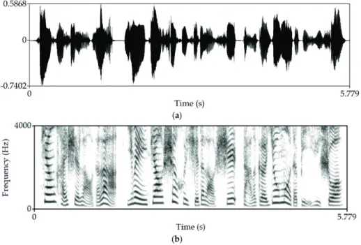
∥X[k, l]∥² are easily interpretable. In Fig. 2.2, it can be seen the spec- trogram of a speech waveform. The horizontal patterns correspond to harmonic frequencies of the voice, which is characteristic of each person.

Figure 2.2: a) Speech waveform and b) its corresponding spectrogram.

Illustration from [Lu et al., 2018].

2.1.3 The Human Auditory System and Mel Spectrogram

Sounds we can hear depend on their intensity and spectrum, and our au- ditory system. STFT, while suitable for ML applications of any kind, is a pure mathematical analysis of the spectrum of a waveform, and does not take into account the human auditory system and mechanisms behind

sound perception. Our auditory system is highly non-linear. Different fre- quencies require different levels of energy to be perceived. Besides, fre- quency perception is interlaced, as described in [O’shaughnessy, 1987]:

“perception of sound energy at one frequency is dependent on the distri- bution of sound energy at other frequencies as well as on the time course of energy before and after the sound”.

Mel scale is an analytical expression of this non-linearity, developed by measuring listeners’ perception to form an equidistant distribution of pitches. Mel scale is depicted in Fig. 2.3. We can observe that humans perceive low frequencies with a higher resolution.

Figure 2.3: Mel scale. Illustration from [Appleton et al., 1975]. The Mel scale’s analytical expression is 2595 log₁₀(1 +f /700), where f is fre- quency (Hz).

Built upon STFT and the aforementioned psychoacoustic findings, mel spectrograms were developed. Mel spectrograms are nothing but a dimensionality reduction carried out with a mel-frequency filterbank. The relationship between a mel-spectrogram,Y, and its former spectrogram is defined by a matrix multiplication,Y_pl = P

kW_pk∥X_kl∥, whereW is the mel filterbank.

Figure 2.4: Mel filterbank (23 filters) as a function of STFT with DFT size 128. Illustration from [Benesty et al., 2008].

2.2 Deep neural networks

2.2.1 The U-Net

The U-Net architecture is a type of CNN that is commonly used for tasks such as image segmentation, image-to-image conversion, audio source separation and others. The U-Net architecture was first introduced in [Ronneberger et al., 2015] for medical image segmentation and owes his name to its characteristic U-shape, as illustrated in Fig. 2.5.

Figure 2.5: Original U-Net architecture [Ronneberger et al., 2015].

The U-Net consists of a contracting path and an expanding path, that act as encoder and decoder, respectively. The contracting path follows the typical architecture of a CNN, with alternating convolutional and pooling layers that progressively reduce the spatial resolution of the input. In the expanding path, the spatial resolution of the feature maps is increased through the use of up-sampling layers. The up-sampling layers are con- catenated with the feature maps from the corresponding layer in the con- tracting path via skip connections, allowing the network to use both high- level semantic information from the contracting path and low-level spa- tial information from the input image. Different modifications have been proposed in different fields and context, for example using strided convo-

lutions instead of max-pooling.

2.2.2 Transformers

A transformer is a type of NN designed as a sequence-to-sequence model.

It maps sequences of any kind and length into other sequences of any kind and length. That is why it has been used in translation, text-to-speech, or image classification among other tasks.

The core idea behind transformers is self-attention and multi-head at- tention. Self-attention is a mechanism used to calculate the relevance of each element in the input sequence with respect to all other elements in the sequence. This is done by projecting the input sequence onto three different vectors called keys, queries, and values; and calculating the sim- ilarity between each query vector and all key vectors. The resulting sim- ilarity scores are used to compute a weighted sum of the value vectors.

Multi-head attention is an extension of self-attention in which multiple self-attention mechanisms are applied to the input sequence in parallel, and the outputs of these mechanisms are concatenated and projected onto a final output vector. This allows the model to learn multiple different representations of the input sequence simultaneously.

The mapping capabilities of the model are given by the “feed-forward”

layer, which is nothing but a multi-layer perceptron applied after attention modules.

There are several advantages to using transformer models in machine learning. Some key advantages of transformers include:

• Improved parallelization: Since the self-attention mechanism cal- culates the relevance of each element in the input sequence with respect to all other elements in the sequence at once, it can be paral- lelized. This allows transformer models to be trained and evaluated much faster than recurrent neural networks.

• Better performance on long sequences: Transformer models are particularly well-suited to processing long sequences of data. This is because self-attention can capture long-range dependencies within

the data from the very beginning. For example, in image classifi- cation, CNNs need depth to reach a proper receptive field; and in text classification, recurrent NNs tend to forget previous elements of sequence through time.

• Better handling of variable-length inputs: The length of the input sequence may vary from one sample to the next. As transformer models do not rely on fixed-sized input representations, they can easily handle variable-length inputs without the need for padding or truncation.

Overall, the use of transformer models in ML can provide significant per- formance benefits, particularly when working with long sequences of data or when dealing with variable-length inputs.

2.3 Visual representations

2.3.1 Motion, graphs, and face landmarks

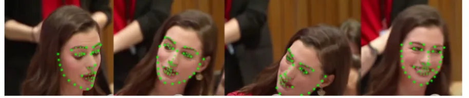
Face landmarks are a set of keypoints in a facial image that correspond to important anatomical features, such as the eyes, nose, mouth, and jaw- line as shown in Fig. 2.6. Face landmarks can be considered as a graph consisting of a set of edges, E, and nodes, V, such that G = (E, V).

V can be defined as V = {vit|i = 1..N;t = 1..T} where i represents the spatial index at the t-th video frame. The set of edges can be decom- posed into temporal edges and spatial edges. Spatial edges are defined as Es = {vitvjt|(i, j) ∈ H}, where H is the set of indices that retains the face shape. Temporal edges connect each landmark with the analogous one in the next frame as follows,E_f ={v_itv_i(t+1)}. This representation is suitable for processing face landmarks with spatio-temporal graph neural networks, which are very good at extracting motion information.

Figure 2.6: Example of landmarks extracted from a high-quality video with large head displacements and broad points of view at 1 FPS. Frames correspond to Anne Hathaway’s speech: Paid Family Leave.

There are many associated advantages in using face landmarks, which alleviate partially or totally many of the challenges mentioned in Sec.

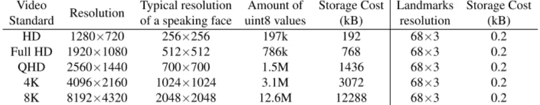
1.2.2. In Table 2.1, the storage cost of different common video standards is shown. The storage cost grows quadratically with video resolution, and so does the computational cost to process each video. Due to the huge amount of information video encodes, we may experience overfit- ting problems, storage shortage, or lack of computational power. The key to solving these is landmarks are a compact and efficient representation

Video

Standard Resolution Typical resolution of a speaking face

Amount of uint8 values

Storage Cost (kB)

Landmarks resolution

Storage Cost (kB)

HD 1280×720 256×256 197k 192 68×3 0.2

Full HD 1920×1080 512×512 786k 768 68×3 0.2

QHD 2560×1440 700×700 1.5M 1436 68×3 0.2

4K 4096×2160 1024×1024 3.1M 3072 68×3 0.2

8K 8192×4320 2048×2048 12.6M 12288 68×3 0.2

Table 2.1: Most common standards in video for 17:9 and 16:9 formats and the storage cost of a single frame. The typical resolution of speaking face is based on a single speaker giving a speech from a tribune. We refer to Anne Hathaway’s speech: Paid Family Leave as an example.

The video can be found at https://www.youtube.com/watch?

v=gkr57P0fwbI

of a person’s face. First, this can make it easier to train NNs and can reduce the amount of data that needs to be processed, which can speed up the training process and reduce overfitting. Second, as we can rep- resent face landmarks as a graph, we can use Graph Convolutional Net- works (GCNs). Unlike images, where the distance among pixels is fixed and structured, the distance among the coordinates of face landmarks can vary. Hence, GCNs can effectively capture the spatial relationships be- tween different nodes with few data. Third, face landmarks drop appear- ance and background information. Therefore, they are robust to varia- tions in lighting and pose, and ensures only pure motion-based features are learned. This increases the models’ privacy, as no additional image information is required. And generalization in terms of gender and eth- nicity. Lastly, the aforementioned face alignment also reduces overfitting and increases generalization to unknown camera’s points of view, which is particularly useful if working with few data.

2.3.2 Audio-visual HuBERT

While face landmarks are a well-suited representation for audio-visual speech tasks, they are still low-level features, encoding raw motion and spatial structure. With the flourishing of machine learning, big tech com-

panies have been developing large-scale models with billions or trillions of parameters. These large-scale models learn powerful representations, closer to human concepts and semantic.

A very good example is Audio-Visual HuBERT. AV HuBERT is a transformer trained to carry out lip-reading and AV speech recognition.

It is trained upon findings from [Devlin et al., 2018] where the authors present a way of obtaining meaningful pre-trained representations for nat- ural language, which led to Bidirectional Encoder Representations from Transformers (BERT). These representations are obtained by a self super- vised training technique called “masked language modeling,” in which a portion of the input text is randomly masked. The model is trained to predict the masked tokens based on the context provided by the remain- ing input text. The model is later fine-tuned for a wide range of down- stream tasks. This training technique was extended to the audio domain in [Hsu et al., 2021]. In that work, the authors run a clustering algorithm on the input acoustic features to generate frame-level assignments (one per sequence element). Then, the model is trained to predict those, also applying the masking strategy from BERT, which forces the model to learn good acoustic features.

AV HuBERT extends this strategy to multimodal data similarly. They incorporate a modality dropout, in which one modality is disabled ran- domly to force the model to solve the task from both modalities. This pre-training strategy and the expressiveness (large amount of parameters) of the network results in very powerful visual and acoustic features, which encode high-level information with semantic meaning.

2.4 Foundations on Sound Source separation

2.4.1 Problem formulation

Blind Source Separation (BSS) is the problem of separating a set of mixed signals into their individual components, without any prior knowledge about the underlying sources or the mixing process. This is in contrast to informed source separation, where additional information about the

sources or the mixing process is leveraged to make the separation process more effective.

In the context of this thesis, the type of signals to isolate are voices and instruments, from which video information is always known. Hence, we are going to bound the problem to music source separation, speech separation, and singing voice separation. While acoustic characteristics are different among them, the way of tackling the separation process is the same when using machine learning. We also assume mono audio, which is predominant in video-streaming platforms.

Given a set of N acoustic signals{x_i(t)|i = 1, ..., N}, we can model a mixture of signals as their linear combination:

x_m(t) =

N

X

i=1

x_i(t).

This is an approximation. In music industry, tracks are mixed with high non-linearity, e.g., when filtering. There exist also natural phenomena such as reverberation that violate this assumption.

Our goal is to recover each independent signal xi(t). This problem is undetermined, as there exists a single observation of the mixture. This problem can be solved with different strategies. In general, when using deep learning, a typical approach is feeding a NN with the mixture and, optionally, other kinds of information that guides the source separation process (one-hot categorical vectors[Slizovskaia et al., 2021], video, text [Rahimi et al., 2022]...).

We can classify the NNs depending on whether they work directly on waveforms, their time-frequency representation, i.e. their STFT, or both (hybrid approaches). Most of the classical algorithms for source separa- tion used to work in the time-frequency domain. Besides, computer vi- sion has traditionally introduced the most advanced architectures in deep learning. As STFT is a 2D signal, those could be easily adapted. There exist some technical reasons as well. Time-frequency representations are more disentangled than time-domain ones. In addition, time-frequency source separation was carried out with a masking system, which is sim- pler (but less powerful) to estimate than a whole signal directly.

2.4.2 Sound Source Separation in the time-frequency do- main

Recalling the notation from Sec. 2.1.2, letx[t]be a generic discrete time audio waveform and X[k, l] be its STFT, where k = 0, ..., K −1 is a frequency index andl = 0, ..., L−1is a frame index.

When working in the time-frequency domain, the usual approach is to predict a mask that acts as a filter by enhancing the target sources.

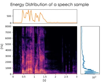
The reasons to do so are two-fold: first, the isolated signals are already present in the mixture, therefore it is possible to isolate them rather than re-synthesize them. Second, energy is usually concentrated in the low- frequencies of the spectrum, as shown in Fig. 2.7. Hence, high frequen- cies would be underrated with Euclidean distances in case of predicting the magnitude STFT directly. Besides, harmonics and structured patterns are weaker in the high frequencies. On the contrary, mask energy is homo- geneously distributed, and a gradient penalty based on the energy of the mixture can be applied. This way, the contribution of each time-frequency bin in the mask to the loss is proportional to the energy of the analogous bin in the mixture.

Masks have quickly evolved. There exist three main types: binary masks, ratio masks, and complex masks. In Eqs. 2.1- 2.4,Mi stands for the mask that isolates the i-th source.

Binary masksrepresent the presence or absence of a particular sound source in the mixture. Each time-frequency bin is set to either 0 or 1. A value of 0 indicates that the corresponding sound source is not present in the mixture, while a value of 1 indicates that it is present. Binary masks predicted by a NN are probability maps, since neural networks cannot generate binary numbers. Binary masks can be formulated in sev- eral ways. In this thesis, two types of binary masks are used: soft binary masks, defined in Eq. 2.1, where each time-frequency point can be as- signed to several sources. And hard binary masks, defined in Eq. 2.2,

Figure 2.7: Energy distribution of a speech sample along frequency and time. Note that the energy distribution along frequency is log-scaled.

where each time-frequency point can be assigned only to a single source.

M_i[k, l] =

(1, if∥Xi[k, l]∥ ≥ ∥Xi[k, l]−Xm[k, l]∥,

0, otherwise. (2.1)

M_i[k, l] =

(1, if∥X_i[k, l]∥ ≥ ∥X_n[k, l]| ∀n ∈ {1, ..., N},

0, otherwise. (2.2)

Ratio masksare another type of masks used in sound source separa- tion. They indicate the relative strength or presence of the sound source in the mixture. Ratio masks are considered a “soft” masking, where the mask is used to attenuate or reduce the strength of a particular sound source in the mixture, rather than completely removing it. Ratio masks can be computed according to Eq. 2.3. Note that, due to the fact it is com- puted as a division between modules of complex numbers, the resulting values can be greater than 1. In practice, the mask is clipped,

M_i[k, l] = ∥X_i[k, l]∥

∥X_m[k, l]∥. (2.3)

Binary and ratio masks are only capable of modifying the magnitude of the spectrogram. In this case, the phase of the mixture is used to recon- struct the isolated waveform. Alternatively, the phase can be estimated with algorithms such as Local Weighted Sums [Le Roux et al., 2010], or GriffinLim [Griffin and Lim, 1984].

More recently, complex maskswere developed. Unlike binary and ratio masks, which only modulate the magnitude, complex masks also modulate the phase. Phase quality is related to robotic effects and natu- ralness, and have proven to improve results in speech separation in works as [Ephrat et al., 2018] or [Williamson et al., 2015]. An implicit formu- lation of complex masks is shown in Eq. 2.4, where⊗denotes complex product. The magnitude of complex masks are unbounded as well. A common approach is using a hyperbolic tangent of real and imaginary parts [Williamson et al., 2015]. This bounds the values and stabilizes gra- dients,

M_i[k, l]⊗X_m[k, l] =X_i[k, l]. (2.4)

2.4.3 Sound Source Separation in the time domain and hybrid approaches

Generally speaking, estimating the phase of a spectrogram is not straight- forward. That is why, concurrently to complex masks, time-domain sound source separation gained attention. The first competitive attempt proposes a 1D U-Net for sound source separation [Stoller et al., 2018]. This ap- proach is data greedy, as 1D CNNs tend to have more parameters due to their large kernels. In addition, the isolated sources were estimated di- rectly, mainly via mean square error or absolute error. This is harder than estimating masks, though potentially more powerful, and incurs the well- known problematic of average-smoothing derived from using Euclidean distances.

Time-frequency domain is more disentangled than time domain. This has very recently lead to hybrid approaches, where NNs are exposed to both, waveforms and STFT in parallel [Rouard et al., 2022].

2.4.4 Sound Source Separation before Deep Learning

While this thesis is focused on deep learning approaches, BSS was al- ready tackled with classical algorithms. Traditionally, BSS in the monoau- ral case (a single microphone) has been approached with matrix decom- position algorithms such as Independent Component Analysis (ICA), e.g.

in [Hyv¨arinen and Oja, 2000], concurrently to ICA, with sparse decom- position [Zibulevsky and Pearlmutter, 2001], Non-negative Matrix Fac- torization (NMF) [Virtanen, 2007], Computational Auditory Scene Anal- ysis (CASA) [Ellis, 1996], or Probabilistic Latent Component Analysis (PLCA) [Smaragdis et al., 2006].

2.4.5 Mix-and-separate Strategy

High-performance, robust ML methods require large amounts of data cov- ering all possible scenarios. If this condition is accomplished, and models are expressive enough, they can generalize pretty well. One of the chal- lenges introduced in Sec. 1.2.2, was related to the difficulty of labeling au- dio data. In real-world acoustic performances, sources are interlaced. On- sets usually happen at the same time, there is reverberation, chorals, sim- ilar tempo etcetera... Collecting real-world ground-truth data implies the capability of recording isolated sources playing at the same time, which is very difficult. There are some attempts from researchers working in mu- sic source separation, where players or singers were recorded in different isolated chambers and synchronized using headphones [Li et al., 2019].

Even following this strategy, it is very expensive to collect large scale datasets.

To overcome the lack of labeled data, the mix-and-separate strategy is often used [Zhao et al., 2018]. Taking advantage of the linearity of the mixtures, an unlimited amount of scenarios can be generated syntheti- cally by combining the sources smartly together with different acoustic resources that emulate real artifacts.

Part I

Audio-visual Source Separation

Chapter 3

INSTRUMENTAL MUSIC

SOURCE SEPARATION