Universidad Católica San Pablo: Foreground detection using attention modules and a video encoding

(1)

COMPUTACI ´ ON

DEPARTAMENTO DE CIENCIA DE LA COMPUTACI ´ ON

Escuela Profesional de Ciencia de la Computaci´ on

Foreground Detection using Attention modules and a Video encoding

Tesis

Presentada por el bachiller

Anthony Alessandro Benavides Arce

Para Optar por el T´ıtulo profesional de:

Licenciado en Ciencia de la Computaci´ on

Asesor: Rensso Victor Hugo Mora Colque

Arequipa, Febrero 2023

(2)

20 %

INDICE DE SIMILITUD

14 %

FUENTES DE INTERNET

11 %

PUBLICACIONES

4 %

TRABAJOS DEL ESTUDIANTE

1 1 %

2 1 %

3 1 %

4 1 %

5 1 %

6 1 %

7 < 1 %

INFORME DE ORIGINALIDAD

FUENTES PRIMARIAS

Submitted to Universidad Católica de Santa María

Trabajo del estudiante

graphics.najjaci.info

Fuente de Internet

hdl.handle.net

Fuente de Internet

www.ijeast.com

Fuente de Internet

arxiv.org

Fuente de Internet

ebin.pub

Fuente de Internet

Yi Wang, Zhiming Luo, Pierre-Marc Jodoin.

"Interactive deep learning method for segmenting moving objects", Pattern Recognition Letters, 2017

Publicación

(3)

unconditional support, to my advisor Rensso for all the time he has invested in me, to all the teachers for their teachings and to my friends who were present at this stage.

(4)

Abbreviations

AtVE-Net Attention based on a Video Encoding Network BS Background Subtraction

CNN Convolutional Neural Network FD Foreground Detection

PDF Gaussian Probability Density Function LSTM Long short-term memory

PBAS Pixel-Based Adaptive Segmenter PWC Percentage of Wrong Classifications

RNN Recurrent Neural Network

TCNN Transposed Convolutional Network

UMBS Universal Multimode Background Subtraction

(5)

Foreground detection is the task of labelling the foreground (moving objects) or background (static scenario) pixels in the video sequence and it depends on the context of the scene. For many years, methods based on background model have been the most used approaches for detecting foreground; however, their methods are sensitive to error propagation from the first background model estimations. To address this problem, we proposed a U-net-based architecture with a feature attention module, where the encoding of the entire video sequence is used as the attention context to get features related to the background model. Furthermore, we added three spatial attention modules with the aim of highlighting regions with relevant features. We tested our network on sixteen scenes from the CDnet2014 dataset, with an average F-measure of 97.84. The results also show that our model outperforms traditional and neural networks methods. Thus, we demonstrated that feature and spatial attention modules on a U-net based architecture can deal with the foreground detection challenges.

Keywords

Foreground Detection, U-Net, Attention, Video Encoding

(6)

La detección de primer plano es la tarea de etiquetar los p´ıxeles de primer plano (objetos en movimiento) o de fondo (escenario estático) en la secuencia de video y esto depende del contexto de la escena. Durante muchos años, los métodos basados en la sustracción de fondo han sido los enfoques más utilizados para detectar el primer plano; sin embargo, sus métodos son sensibles a la propa- gación de errores a partir de las primeras estimaciones del modelo de fondo.

Para abordar este problema, proponemos una arquitectura basada en U-net con un módulo de atención de caracter´ısticas, donde la codificación de toda la secuencia de video se usa como contexto de atención para obtener caracter´ıs- ticas relacionadas con el modelo de fondo. Además, añadimos tres módulos de atención espacial con el objetivo de resaltar las regiones con caracter´ısti- cas relevantes. Probamos nuestro modelo en dieciséis escenas del conjunto de datos CDnet2014, con un puntaje F-measure promedio de 97.84. Los resulta- dos también muestran que nuestro modelo supera los métodos tradicionales y de redes neuronales. Por lo tanto, demostramos que los módulos de atención espacial y de caracter´ısticas en una arquitectura basada en U-net pueden hacer frente a los desaf´ıos de la detección de primer plano.

Palabras clave

Foreground Detection, U-Net, Attention, Video Encoding

(7)

List of Tables

5.1 Scenes from the CDnet2014 with their size and the number of frames [Ak- ilan et al., 2019]. . . 31 5.2 F-measure performance comparison. In this table, we present the compar-

ison on sixteen CDnet2014 scenes of our vanilla model and our AtVE-Net method against PBAS [Hofmann et al., 2012], UMBS [Sajid and Cheung, 2017], DeepBS [Babaee et al., 2018] and 3D-LSTM [Akilan et al., 2019].

n/a means that the result was not available. The scores of the PBAS, UMBS and DeepBS methods were acquired from [Akilan et al., 2019]. . . . 33 5.3 Performance comparison with PWC. In this table, we present the compari-

son on eight CDnet2014 categories of our vanilla model and our AtVE-Net method against UMBS [Sajid and Cheung, 2017], DeepBS [Babaee et al., 2018], 3D-LSTM [Akilan et al., 2019] and U-Net MDI [Kim and Ha, 2021].

n/a means that the result was not available. The scores of the PBAS, UMBS and DeepBS methods were acquired from [Akilan et al., 2019]. . . . 33 5.4 F-measure performance comparison with one, two and three spatial atten-

tion modules in our AtVE-Net architecture. These experiments were performed on eight CDnet2014 categories using the spatial attention modules from the third skip-connection to the first skip-connection. . . 34 5.5 PWC performance comparison attention with one, two and three spatial

attention modules in our AtVE-Net architecture. These experiments were performed on eight CDnet2014 categories using the spatial attention modules from the third skip-connection to the first skip-connection. . . 34

(11)

List of Figures

2.1 Background subtraction modules [Babaee et al., 2018]. . . 7 2.2 Gaussian mixture with the mean µ, the covariance σ and the clusters of

points. . . 8 2.3 A representative Convolutional Neural Network (CNN) architecture. . . 9 2.4 A convolution and a transposed convolution operations. A convolution

kernel is positioned over each pixel of an input feature map to be convolved generating an output feature map. . . 10 2.5 Activation functions. We present sigmoid, tanh and ReLU activation func-

tions. . . 11 2.6 Pooling function. . . 12 2.7 Comparison of 2D and 3D convolution operations [Gao et al., 2018] . . . . 13 2.8 A standard LSTM module with three gates. The input and forget gates are

used to calculate the cell state c_t. The cell state and the output gate are used to calculate the hidden state h_t. The symbol∽ means tanh function.

The symbol × denotes the Hadamard product. . . 14 2.9 Scaled dot-product attention [Vaswani et al., 2017]. . . 15 2.10 U-net architecture [Ronneberger et al., 2015]. . . 16 2.11 ResNet-34 architecture [He et al., 2016]. At the bottom, each residual block

is detailed with the size of the kernel and the number of filters. At the top of each residual block indicates the number of repeated blocks. Finally, the model applies an average pooling, a fully connected layer and a softmax function. . . 16 3.1 Overview of the Pixel-Based Adaptive Segmenter[Hofmann et al., 2012]. . . 19 3.2 Overview of the PSPnet Architecture [Zhao et al., 2017]. . . 21 3.3 Overview of the BSUV-Net Architecture [Tezcan et al., 2019]. . . 22

(12)

3.4 A layer-wise schematic of the 3D CNN-LSTM architecture [Akilan et al., 2019]. . . 23 4.1 Overview of AtVE-Net architecture. We highlight U-net architecture, in-

cluding its encoder, decoder and skip-connections. We also highlight the attention modules and the video encoding, which are our main contributions. 25 4.2 Our feature attention module takes the high representation of the features

z. This module consists of two steps: i) We disentangled z to generate independent representations, in order to attend various aspects of the latent space where we apply layer normalization [Ba et al., 2016] to it. ii) Then, we generate the attention maps using linear transformations on the disentangled output to obtain the value V and key K, and we use the video encoding as input for the query value Q. This results in the feature selection from the disentangled output. In the figure, AAP means adaptive average pooling. . . 27 4.3 Our spatial attention module takes the feature representation obtained in

the feature attention module z, and the feature maps coming from the skip- connection of the network x. We apply layer normalization [Ba et al., 2016]

to z and x. Then, we generate the attention maps using linear transformations on x to obtain the value V and key K, and we use z as input for the query value Q. Finally, we apply a linear layer to generate the resulting feature maps. This results on the highlights of regions with relevant features. 28 4.4 Vanilla AtVE-Net architecture. Vanilla AtVE-Net is based on a U-net ar-

chitecture. We present the encoder and decoder feature maps with green and white color, respectively. Unlike vanilla U-net, we add a feature attention module on the last encoder layer and a visual encoding as an attention context. Thus, the attention module is able to select features with useful information for FD. Finally, the last network layer has a sigmoid activation function because the network output is going to label each pixel with a probability between 0 and 1 in order to distinguish between background and foreground, respectively. . . 29 4.5 AtVE-Net architecture. AtVE-Net is based on our vanilla model architec-

ture. We present the encoder and decoder feature maps with green and white color, respectively. The yellow feature maps represent the resulting attended features from the spatial attention module. Unlike our vanilla model, AtVE-Net incorporates spatial attention modules on the last three skip-connections. Finally, the last network layer has a sigmoid activation function because the network output is going to label each pixel with a probability between 0 and 1 in order to distinguish between background and foreground, respectively. . . 29 5.1 Qualitative results of the proposed model. We divide our qualitative re-

sults in blocks of three images: the input frame, the ground-truth and the foreground segmentation obtained from AtVE-Net model. . . 36

(13)

5.2 Attention maps obtained by the spatial attention module in AtVE-Net.

For each scene we present the input frame, ground-truth, and the attention maps obtained from the spatial attention module in the third skip- connection of our AtVE-Net model. Note that we changed the black pixels to white pixels to have a better identification of the attention maps. . . 37

(14)

Chapter 1 Introduction

1.1 Motivation and Context

With millions of hours of videos recorded daily in the world, it is only needed the highlights of video sequences to perform multiple surveillance tasks including object tracking, traffic monitoring, anomaly detection, action recognition, traffic analytic, video compression, etc.

[Wang et al., 2017]. To this end, Foreground Detection (FD) is a widely used approach, it is a binary classification task which assigns each pixel in video sequences with labels belonging to foreground and background. Foreground is defined by [Lim and Keles, 2018]

as the moving objects in the scene, in our context, foreground are the objects that do not belong to the scene. On the other hand, the background is the static scenery. FD is used as a pre-processing step in applications like hand gesture identification [Hema, 2016], video compression [Wu et al., 2020], segmentation [Tarafdar et al., 2019] and vehicle counter [Fratama et al., 2019].

FD remains a challenging task due to various factors in video sequences as: (1) Illumination changes, caused by the variation of lighting in the scene due to changes in the lights or changes in the brightness of the sun. (2) Dynamic background, due to possible background changes during the scene, especially in outdoor scenes, e.g. waves or swaying tree leaves. (3) Camera jitter, due to a motion camera, the background is not static. (4) Camouflage, it is when the foreground is falsely labelled as background because they have similar color [Babaee et al., 2018]. The main challenge of FD is to be able to distinguish the dithering effect at the boundaries of foreground objects, overcoming the previous challenges.

The most used method for FD is the Background Subtraction (BS) technique. It defines the foreground by extracting the difference between the current frame and the background. This technique consists of two stages: 1) an estimation of the background model from the video sequence and 2) foreground extraction by subtracting the background model [Huynh-The et al., 2016]. In this context, a background model consists of a reference to compare against input frames. Background subtraction is a complex and subjective task because it can fall into the propagation of errors due to a poorly estimation of the background model and there is a large amount of temporal information

(15)

between adjacent frames, nevertheless, state-of-the-art methods do not take advantage of the context provided by a background model [Lim and Keles, 2018, Sajid and Cheung, 2017, Akilan et al., 2019]. We expect that a video encoding of the total sequence of frames is better than employing a background model methodology. And we use attention modules to obtain the abnormal features of the current frame by comparing it with the features obtained from the video encoding.

The state-of-the-art methods of FD employ a robust benchmark called CDNet2014 [Wang et al., 2014b]. This dataset is widely used because it presents eleven different categories with various frame sequences per category and their ground-truth. Our method was tested on sixteen scenes from the CDNet2014 dataset, with F-measure and percentage of wrong classifications (PWC) metrics. It was a challenging dataset because each scene has a variety of challenges including a dynamic background, night videos, intermittent object motion, etc. Our model is obtaining an overall F-measure of 97.84 and PWC score of 0.20, outperforming the evaluated methods.

This thesis focuses on visual surveillance in order to detect and track moving objects, and interpret their activities and behaviors [Maddalena and Petrosino, 2008]. The use of FD to this aim could be from videos recorded from stationary camera as in [Stauffer and Grimson, 1999, Sheikh and Shah, 2005, Ko et al., 2010] and non-stationary camera as in [Moo Yi et al., 2013, Yun and Choi, 2015]. This work deals with the FD of environments captured from a stationary camera where the essential conditions of the scene do not change, e.g. if our model performs FD on road cars, it cannot be adapted to detect cows on a green field. We employ video sequences with video resolution greater than or equal to 240×320 pixels and a frame rate greater than or equal to 25 fps.

1.2 Problem Statement

Dealing with FD is a difficult task, due to there is a large amount of temporal information between adjacent frames in video sequences, nevertheless, the compared methods do not take advantage of the maximum potential that temporary information offers in the FD task. Although the neural network methods have different approaches, they segment the foreground objects with a dithering effect in the boundary. Also, the state-of-the-art methods are not taking advantage of the context provided by a background model. The challenge addressed in this thesis deals with time-dependent motion using a background model approach, while keeping the main FD challenge resolved.

1.3 Hypothesis

Background subtraction is a complex and subjective task because it can fall into error propagation due to poor estimation of the background model. Based on the researches of [Lim and Keles, 2018, Sakkos et al., 2018, Akilan et al., 2019], our approach does not need to update the background model and use it to subtract the current input frame.

Instead, we employ a background model approach as a context guide to highlight objects

(16)

that do not belong in the scene. Therefore, we propose a model based on the U-net architecture [Ronneberger et al., 2015] that allows the network to incorporate global and local features. In addition, we employ a video encoding and two attention mechanisms:

(i) A feature attention module to process the high encoding of U-net and compare it with the features obtained from the video encoding and, (ii) spatial attention modules on the skip-connections of the network with the aim of highlighting regions with relevant features [Flores-Benites et al., 2021], where we would use the feature representation obtained in the feature attention module in order to recognize the spatial regions where these features are found. As a result, our model projects the video information into a latent space, where has rich spatial and temporal information.

1.3.1 General Objective

The main objective is to generate a model that employs attention modules and a video encoding of the entire video sequence to perform the Foreground Detection task.

1.3.2 Specific Objectives

1. Design and implement a U-net based model with attention modules and a video encoding that deals FD.

2. Analyze and compare the proposed model with only the feature attention module and the model with the addition of the spatial attention modules.

3. Test and validate the correct operation of the proposed method.

4. Perform an ablation study on the spatial attention modules of our model.

1.4 Contributions

We present a model that employs spatio-temporal information, and it does not need a background model to define the foreground. Our model exploits the capacity of attention modules to highlight irregularities and a context provided by a video encoding of the entire video sequence. Our main contributions are:

1. We introduce a non-updatable background model approach as a context. To this end, we use the features obtained from encoding the entire video sequence.

2. We use a feature attention module to detect irregularities by comparing the current input features and the scene context.

3. We use spatial attention modules to recognize the irregularities in the up-sampled steps using the features obtained in the feature attention module.

(17)

4. This research carried out a publication on ICIAP 2021 Conference Proceedings, with the name of Foreground Detection using an Attention module and a Video encoding [Benavides-Arce et al., 2022].

The remaining chapters of this thesis are organized in five chapters: The Chapter 2 comprises a review of the basis of the concepts seen in this work. In the Chapter 3, the related state-of-the-art of FD is presented with a brief explanation of the models and the considerations related to them. In the Chapter 4, the proposal of a FD model that employs attention modules and a video encoding is presented. In the Chapter 5, the tests and results obtained from our model are presented. Finally, in the Chapter 6, the conclusions of this thesis are exposed.

(18)

Chapter 2

Theoretical Foundations

This chapter comprises a review of the main theoretical foundations seen in FD and BS.

In particular, the fundamentals of BS, concepts of statistical and linear algebra, and the fundamentals of convolutional neural networks.

2.1 Fundamentals of Background Subtraction

BS is a widely used approach to detect foreground objects, in this section we describe the main concepts of BS such as the processing modules of BS and the post-processing thresholds used in BS and FD methods.

2.1.1 Background Subtraction Modules

The BS pipeline has four processing modules, which are not all essential [Babaee et al., 2018]. The four processing modules are: (I) Background Model: This is a reference map used to compare with the input frames to detect foreground objects. An important step for the background model is the initialization without foreground objects. (II) Feature extraction: This step compares the background model with the input frames, the model selects the relevant information features. (III) Background Model Maintenance:

The background changes over time, therefore, it needs to be updated; usually, this step employs the previous segmentation outputs. To perform background model maintenance, it is critical to select an adequate adaption rate of the background model maintenance in order to update the background over time and not to update foreground objects. (IV) Segmentation: It extracts the features of the corresponding pixel regions from the frame and the background model. Usually, euclidean distance is used to measure the similarity between those pixels. Finally, the resulting segmentation is compared with a threshold, where each pixel is labeled as foreground or background [Babaee et al., 2018]. The entire pipeline can be seen in Fig. 2.1.

(19)

Background Maintenance

Feature Extraction Input Frame

Background Model

Background Segmentation Segmentation

Background Maintenance

Feature Extraction

Background Model

Segmentation

Figure 2.1: Background subtraction modules [Babaee et al., 2018].

2.1.2 Thresholds of Foreground Detection and Background Subtraction

Threshold is a post-processing step of the FD and BS models. It is located just after the segmentation module. The segmentation module outputs a probability between 0 to 1 to belong to a background or foreground respectively. If the output probability is greater than the threshold, it is labeled as foreground and otherwise as background. The choice of the threshold value for the background subtraction is important to achieve the significant motion detection [McIvor, 2000].

Thresholds of FD are classified according to their variation over time, if the threshold is updated or not. There are two types of thresholds:

• Static threshold: It never changes, it remains over time and is a single value, usually obtained by trying different threshold values and the best value remains as the static threshold. Methods of FD that implement this kind of threshold are [Lim and Keles, 2018, Tezcan et al., 2019].

• Adaptive threshold: These thresholds are updated through the time to get better accuracy in the post-processing step. Methods of BS that implement adaptive threshold are [Hofmann et al., 2012, Boufares et al., 2016, Mandal et al., 2018, Hanchina- mani et al., 2016, Bennet et al., 2017].

2.2 Statistical and Linear Algebra Concepts

Statistical and linear algebra concepts, including Gaussian mixture and eigenvectors, are described to provide background for the handcrafted methods detailed in the next chapter.

(20)

2.2.1 Gaussian Mixture

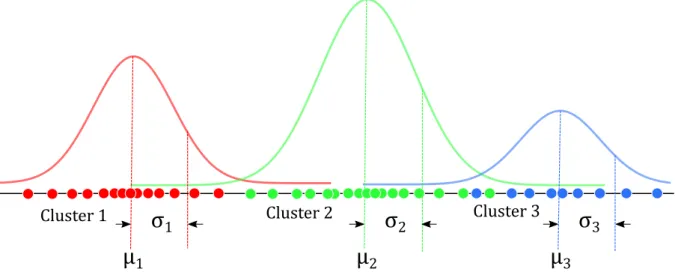
A Gaussian Mixture is a Gaussian Probability Density Function (PDF) comprised of many Gaussian distributions [Bishop and Nasrabadi, 2006]. A probability density function is a statistical expression that defines a probability distribution or the likelihood of an outcome. A PDF can describe either discrete or continuous data, the difference is that discrete variables can only take on specific values, such as integers, yes or no, times of day, etc.; on the other hand, continuous variables are comprised of an uncountable set.

Each Gaussian distribution is identified by k∈1, . . . , K, whereK is the number of clusters in our points. Each Gaussiank has a mean, a covariance and a mixing coefficient.

The mean µ is the center, the covariance σ is the width of the curve and the mixing coefficient π is a probability to each Gaussian distribution. The sigma coefficient must meet this condition:

K

X

k=1

πk = 1, (2.1)

in the Fig. 2.2, we can see a Gaussian mixture with its main components.

μ

₁

σ

₁

Cluster 1 Cluster 2 Cluster 3

μ

₂

σ

₂

μ

₃

σ

₃

Figure 2.2: Gaussian mixture with the meanµ, the covarianceσand the clusters of points.

2.2.2 Eigenvectors and Eigenvalues

Eigenvectors and eigenvalues are linear and homogeneous equations [Weisstein, 2002]. Let V be a vectorial space over a field F and let T be a linear transformation T : V → V, there are vectorsv for which there exists a value such thatT(v) =λv. An eigenvalue of a linear transformation T is a scalarλ, such that (λI−T) is not invertible. An eigenvector of T is a vector v different from 0 that satisfies (λI −T)v = 0. For example, for the transformation T(x, y, z) = (−2x+ 15y+ 18z,3y+ 10z, z), we observe that:

(21)

T(1,0,0) = (−2,0,0)

=−2(1,0,0)

T(3,1,0) = (−6 + 15,3,0)

= (9,3,0)

= 3(3,1,0),

(2.2)

where (1,0,0) and (3,1,0) are eigenvectors ofT with eigenvalues of−2 and 3 respectively.

To each eigenvector corresponds an eigenvalue. Eigenvectors and eigenvalues are used in Principal Component Analysis (PCA) method [Bishop, 1998], each of the components corresponds to an eigenvector, and the component order is established by decreasing order of eigenvalue. Thus, the first component is the eigenvector with the highest associated eigenvalue.

2.3 Fundamentals of Convolutional Neural Networks

Convolutional Neural Networks (CNNs) have many applications in image processing.

Deep CNNs can learn hierarchical features from input images, where features at higher levels are more abstract than those at lower levels. Typically, CNNs contain three elements: a convolutional layer, a pooling layer and an activation function. These elements are joined together to form a convolution block and deep-level architectures have several of these blocks [Zhou et al., 2020]. Figure 2.3 shows a representative CNN architecture.

Input Feature maps

Convolution Pooling Convolution Activation Function Figure 2.3: A representative CNN architecture.

2.3.1 Convolution Operation

CNNs has as a main component the convolution operation. A convolution is an integral that expresses the amount of overlap of one function g(x) as it is shifted over another function f(x). In one dimension, the convolution of two continuous functions f(x) and g(x) produces a third function [McReynolds and Blythe, 2005]:

(22)

h(x) =f(x)∗g(x) = Z +∞

−∞

f(τ)g(x−τ)dτ, (2.3)

where g(x) is referred to as the filter. The integral only needs to be evaluated over the range whereg(x−τ) is non-zero. The discrete form of convolution operates on two arrays, the discretized signal F[x] and the convolution kernel G[0. . .(width−1)]. The value of width defines the support of the filter and equation 2.3 becomes:

H[x] =

width−1

X

i=0

F[x+i]G[i], (2.4)

the one dimensional discrete form is extended to two dimensions as:

H[x][y] =

height−1

X

j=0

width−1

X

i=0

F[x+i][y+j]G[i][j] (2.5)

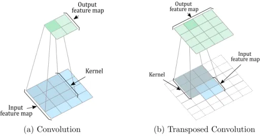
For a better understanding, we present Fig. 2.4a, where a convolution kernel is positioned over each pixel of an image to be convolved. Multiplying and summing the kernel against the pixels covered in the image creates a new pixel value, which is used to update the output feature maps. The significance of convolution in the spatial domain is that it is equivalent to multiplying the frequency domain representations of the two functions. This means that a filter with some desired properties can be constructed in the frequency domain and then converted to the spatial domain to perform the filtering.

Input feature map

Output feature map

Kernel

(a) Convolution

Kernel

Input feature map Output

feature map

(b) Transposed Convolution

Figure 2.4: A convolution and a transposed convolution operations. A convolution kernel is positioned over each pixel of an input feature map to be convolved generating an output feature map.

(23)

2.3.2 Activation Functions

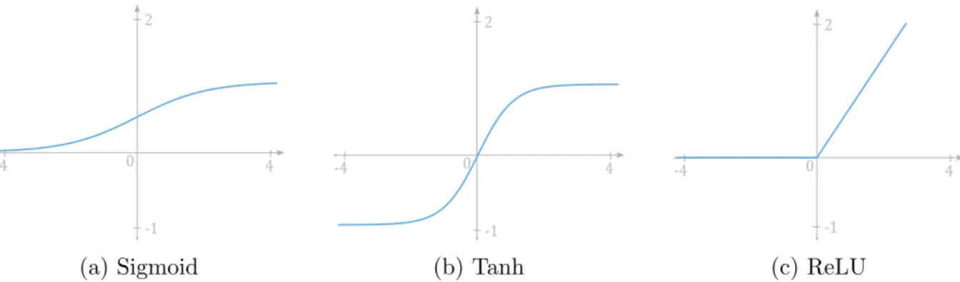
The activation functions provide non-linearity to the output of the inner layers so that it can be further processed because in the real world errors have non-linear characteristics [Sharma et al., 2017]. The prediction accuracy of a neural network is defined by the type of activation function used. For the background of this thesis, we show four activation functions in Fig. 2.5 and we describe them below:

-4 4

2

-1 0

(a) Sigmoid

-4 4

2

-1 0

(b) Tanh

-4 4

2

-1 0

(c) ReLU

Figure 2.5: Activation functions. We present sigmoid, tanh and ReLU activation functions.

• Sigmoid Activation Function: It is the most widely used activation function. Sig- moid function transforms the values in the range 0 to 1. It can be defined as:

f(x) = 1

e^−x (2.6)

• Tanh Activation Function: It is Hyperbolic Tangent function. Tanh function is similar to the sigmoid function, but it is symmetric to around the origin. Tanh values lies in the range −1 to 1. It can be defined as:

f(x) = 2sigmoid(2x)−1 (2.7)

• ReLU Activation Function: ReLU is more efficient than other functions because as all the signals are not activated at the same time. In some cases, the value of gradient is zero, due to which the weights and biases are not updated during back-propagation step in neural network training.

f(x) = max(0, x) (2.8)

• Softmax Activation Function: Softmax function is a combination of multiple sigmoid functions. As we know that a sigmoid function returns values in the range 0 to 1, these can be treated as probabilities of a particular class data points. Softmax function, unlike sigmoid function which is used for binary classification, can be used

(24)

for multi-class classification problems. The function, for every data point of all the individual classes, returns the probability. It can be expressed as:

σ(z)_j = e^z^j Pk=1

K e^z^k for j = 1,. . . ,K. (2.9)

2.3.3 Pooling Function

A typical layer of a CNN consists of three stages. In the first stage, the layer performs several convolutions in parallel, then, a pooling function and a non-linear activation function are applied. Pooling helps to make the representation approximately invariant to small translations of the input. Invariance to translation means that if we translate the input by a small amount, the values of most of the pooled outputs do not change [Goodfellow et al., 2016].

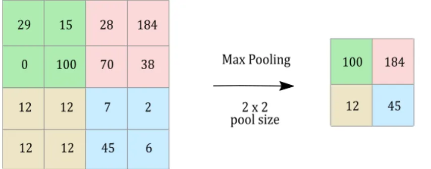
A pooling function replaces a feature map at a certain location with a summary statistic of the nearby outputs. We highlight three approaches of pooling functions: (i) Max pooling, where the maximum pixel value of the batch is selected. (ii) Min pooling, where the minimum pixel value of the batch is selected. (iii) Average pooling, where the average value of all the pixels in the batch is selected. The batch means a group of pixels of size equal to the filter size and the output of the pooling function varies according to the filter size. In the Fig. 2.6, we show a max pooling with a filter of 2×2.

29 15 28 184

0 100 70 38

12 12 7 2

12 12 45 6

100 184

12 45

Max Pooling

2 x 2 pool size

Figure 2.6: Pooling function.

2.3.4 Transposed Convolution Operation

Transposed convolution is not the inverse process of convolution operation; however, it restores the spatial dimensions of the feature maps but not their parameters [Zhou et al., 2020]. In contrast to the regular convolution that reduces input elements via the kernel, the transposed convolution broadcasts input elements via the kernel, thereby producing an output that is larger than the input. We can see how a transposed convolution works in Fig. 2.4b.

(25)

2.3.5 Three-Dimensional Convolution Operation

The 2D convolution operator is used only to extract features from the spatial dimension. The three-dimensional convolution operation aims to extract features from multiple frames, capturing the spatial-temporal information [Gao et al., 2018]. The 3D convolution employs a 3D kernel over stacked frames. Stacked frames usually are a consecutive frames of a video sequence, thus the 3D convolution captures temporal information. Formally, the 3D convolution operation is given in equation 2.10.

a_ji =f(b+

n

X

k=1 x

X

j=1 y

X

i=1

w_kjia_kji), (2.10)

where f(x) is the activation function, b is the bias,wkji is the weight of the j-th row and i-th column for the k-th frame, and a_ji is the output. A graphical comparison between 2D and 3D convolution operation is presented in Fig. 2.7.

2D convolution 3D convolution

temporal

Figure 2.7: Comparison of 2D and 3D convolution operations [Gao et al., 2018]

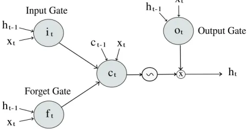
2.3.6 Long Short-Term Memory

Recurrent Neural Network (RNN) [Levin, 1990] allows neural networks to be influenced by past inputs. Long short-term memory (LSTM) is an enhanced version of RNN to have the ability to choose to learn from recent prior information, and it solves the vanishing gradient problem in backpropagation [Gers et al., 1999]. This capability is important since information in the past can be noisy and distort the current result; however, there are cases where we need a context information [Trinh et al., 2016].

An LSTM cell contains a cell state and three different gates: input, output, and forget gates. Each gate is described below:

(26)

• The input gateblocks some features from the current input to update the cell state.

• The output gateis aimed to block some features of the cell state in order to calculate the next hidden state.

• The forget gate decides which information from the input and the hidden state should be remembered and which can be ignored.

The cell state obtains information from the forget gate and input gate. It multiplies the forget gate output to ignore non-relevant signals and uses the input gate result to update the cell state with the signals from the current input. The cell state is used to calculate the output vector. A general representation of a LSTM is presented in Fig. 2.8.

Forget Gate

c

t

c

t-1

i

t

o

t

h

t

f

t

x

Output Gate Input Gate

x

t

x

t

h

t-1

h

t-1

x

t

h

t-1

x

t

Figure 2.8: A standard LSTM module with three gates. The input and forget gates are used to calculate the cell state ct. The cell state and the output gate are used to calculate the hidden state h_t. The symbol ∽ means tanh function. The symbol × denotes the Hadamard product.

2.3.7 Attention

Attention is the use of the human visual system in neural networks [Soydaner, 2022].

Therefore, visual attention has the aim to restrict the processing of the entire input to a subset of the visual field. Attention seeks to find what and where is the relevant information of the input.

The attention mechanism has been improved over the years, therefore, we emphasize the attention mechanism in neural networks. We use the approach proposed by [Vaswani et al., 2017], it is called scaled dot-product attention. It employs a query, key and value vectors for each input. These three vectors are obtained by the multiplication of the input with weight matrices W_q,W_kand W_v which are learned during training. A dot-product is computed between the query and key vectors, and the result vector is divided to the square root of the dimension of the keys to have more stable gradients. The obtained vector is computed in a softmax function. Finally, the resulting softmax score is multiplied with the value vector. It can be seen in Fig. 2.9.

(27)

FCFCFC

z'

Softmax

Scale

z' Q

K

V

Figure 2.9: Scaled dot-product attention [Vaswani et al., 2017].

2.4 Neural Network Architectures

In this section, we describe the neural network architectures pertinent to this thesis. We present encoder-decoder, U-net and ResNet architectures.

2.4.1 Encoder-Decoder Architecture

This is a widely employed architecture in segmentation tasks. The encoder receives the input, it encodes the fixed-dimensional vector into a feature vector, and the decoder employs the feature vector to get the output [Chen et al., 2019]. This architecture can use CNN and/or just RNN in the encoder or decoder. Any combination can be used which is suitable for the given task, as in [Akilan et al., 2019, Lim and Keles, 2018]. The most used encoder-decoder architecture is using CNN.

2.4.2 U-net Architecture

The U-net architecture [Ronneberger et al., 2015] achieved very significant performance in segmentation applications. The U-net encoder includes three blocks of two 3 × 3 convolutions, a rectified linear unit (ReLU), and max poolings 2×2 with stride 2, to down-sample the input. The resulting latent space is feature-rich and is up-sampled with three blocks of 2×2 up-convolution, two 3×3 convolutions, and a ReLU. Each input of the decoder blocks is concatenated with the output of its respective encoder block.

Finally, a 1×1 convolution is used to map each feature vector to the number of output classes. U-net architecture is shown in Fig. 2.10.

(28)

Feature maps

MaxPool 2x2 UpConv 2x2 Copy and crop Conv 3x3+ReLU

Input Output

Figure 2.10: U-net architecture [Ronneberger et al., 2015].

2.4.3 ResNet

Residual Network [He et al., 2016] deals with the degradation problem on deeper networks.

ResNet uses convolution blocks with the same identity mapping and the shallower layers are copied to them, it is called deep residual learning framework. The ResNet pipeline is based on the VGG network [Simonyan and Zisserman, 2014b], the convolutional layers have filters of 3 ×3 except for the first one which has filters of 7 ×7. For the same block, the layers have the same number of filters, and when the feature map is halved, the number of filters doubles to preserve complexity in layers with many filters. ResNet has a good generalization performance on recognition tasks. ResNet-34 architecture is shown in Fig. 2.11.

Image Output

X3 X4 X6 X3

7x7, 64 3x3, 64 3x3, 128 3x3, 256 3x3, 512 Average Pool,

fc and softmax

Figure 2.11: ResNet-34 architecture [He et al., 2016]. At the bottom, each residual block is detailed with the size of the kernel and the number of filters. At the top of each residual block indicates the number of repeated blocks. Finally, the model applies an average pooling, a fully connected layer and a softmax function.

(29)

Chapter 3

Related Work

Several methods for performing FD have been proposed in the literature. The following sections list a set of methodologies that solve the FD problem and we classify them into handcrafted and neural network models. In addition, we present the justification of our research in each methodology.

3.1 Handcrafted methods

Handcrafted methods estimate effectively the background model from the sequence of frames. Usually, these methods segment the foreground objects by differentiating the background model (background image) with the input frame. They generally work at pixel level of the frame and use effective statistical methods [Piccardi, 2004]. These models aim to maximize speed performance. In this section, we describe basic methods such as running Gaussian average, up to methods with complex background models.

A BS basic approach is to run the Gaussian average. It employs a Gaussian PDF at each pixel location, it is described in equation 3.1.

µ_t=αI_t+ (1−α)µt−1, (3.1)

where I is the current pixel value, µ_t is the average value and α is an empirical weight to adjust the update rate. When the difference between the pixel value and the median is less than the variance, the pixel is labeled as foreground [Wren et al., 1997]. [Koller et al., 1994] improved the previous model by updating the Gaussian PDF only when it is a background pixel, it is described in equation 3.2.

µ_t =M µt−1+ (1−M)(αI_t+ (1−α)µt−1), (3.2)

(30)

where M is 1 when the pixel is foreground and 0 otherwise. These methods do not adapt their background model when the background is dynamic.

To deal with the dynamic background problem, models such as [Lo and Velastin, 2001, Cucchiara et al., 2003] employ a temporal median filter, these methods create the background model from the median value of the last n frames. The main drawback is that they require saving the pixels of the last n seen frames and do not use a deviation measure to adapt the subtraction threshold. The same problem has [Stauffer and Grimson, 1999, Power and Schoonees, 2002], they proposed the use of mixture of Gaussians to model the background in three distributions for RGB colors. The Gaussian distributions are described in equation 3.3.

P(xt) =

K

X

i=1

η(xt−µi,t,Σi,t), (3.3)

where K is the number of distributions, in this case K is three for RGB colors, µ_i is the median value and Σi is the covariance matrix. The parameters of these models are difficult to update and adjust to the best distribution. To overcome this, the model of [Elgammal et al., 2000] employs a similar approach to mixture of Gaussians; however, it uses the last 100 seen frames instead of the sum of Gaussians; and the update order is first in, first out (FIFO). However, the last 100 frames viewed may contain foreground objects, so it is not desirable to use FIFO as the update mechanism. The methods of [Comaniciu and Meer, 2002, Comaniciu, 2003] proposed the use of mean shift vector to update the frames used in the model. However, these models have high computational cost within the handcrafted methods.

The models of [Han et al., 2004, Oliver et al., 2000] do not use only the last seen frames, instead they use the spatial correlation. They compute the eigenvectors of the covariance of n frames. For labeling as background or foreground, they compute the eigenvector of the input frame. The model of [Han et al., 2004] labels the pixels as background only if the input frame eigenvector is close to an eigenvector of the background model. The method of [Oliver et al., 2000] back-projects the input frame eigenvector to the original dimensions, then computes the difference with the input frame and thresholds each pixel to label them as background or foreground. The problem with these methods is whether and how the model should be updated.

Pixel-Based Adaptive Segmenter (PBAS) [Hofmann et al., 2012] uses a background model defined by an array of n recently observed background pixel values. For the background model maintenance, PBAS only updates if there is no drastic background change in the current pixel x_i to avoid adding foreground objects to the background model. If it is updated, PBAS chooses uniformly, with probability R(x_i), one of the n samples of the pixel in the background model, replacing it with x_i. T(x_i) and R(x_i) are dynamically updated according to background dynamics. Finally, to reduce noise and spatial smooth- ing, it uses a simple median filtering and labels each pixel independently. The overview of PBAS is presented in Fig. 3.1. PBAS employs an adaptive threshold and an adaptive update rate, such that, the FD get better foreground boundaries; however, PBAS has to update two key parameters in each iteration.

(31)

Input Image (xi) Segmentation Background Decision

Background Model Background Maintenance

Update T(xi) - Decision Threshold

Update R(xi) - Update Rate

Figure 3.1: Overview of the Pixel-Based Adaptive Segmenter[Hofmann et al., 2012].

A similar model is SuBSENSE [St-Charles et al., 2014], it employs the same background model and maintenance as PBAS. Unlike PBAS, SuBSENSE employs a Local Binary Similarity Pattern (LBSP) feature in addition to the RGB values. The LBSP computes the sum of the similarity between the current pixel and its neighbors on a 5×5 grid centered on the current pixel. In this context, the LBSP similarity is 1 if the difference between the two values is less than a threshold and 0 otherwise. The LBSP features in SuBSENSE are often too sensitive to local changes in dynamic and noisy regions, and like PBAS, SuBSENSE has to update two key parameters at each iteration.

Universal Multimode Background Subtraction (UMBS) [Sajid and Cheung, 2017]

uses multiple background models. For the background model maintenance, UMBS employs a linear function that determinates update rate based on the rate of change of the number of foreground pixels in the current frame and the running mean. In the segmentation step, UMBS uses Mega-Pixel formation, which is a cluster of related pixels to reduce spatial noise. The average probability estimation makes clusters of the same object and therefore increments segmentation accuracy. The problem with UMBS is the accuracy drops in the generation of the Mega-Pixels.

3.2 Neural Network methods

These methods are the most accurate in the last few years. Neural network methods generate statistical patterns from training with sample data, the obtained patterns are used to classify new samples [Specht, 1990]. They are sophisticated FD models that assure robust FD. In this section, we present 3D CNN, Multi-Scale CNN, Encoder-Decoder CNN, RNN and Attention Neural Network methods.

(32)

3.2.1 Hybrid CNN methods

Hybrid methods combines handcrafted or statistical methods and a CNN method to achieve the FD. The model proposed by [Simonyan and Zisserman, 2014a] is composed of two streams of CNN, one stream performs spatial information and the other performs temporal information. The spatial stream receives a single frame and the temporal stream takes a sequence of optical flow frames, finally, their outputs are combined by a fusion method. Their model takes spatial and temporal information to perform the action recognition task, nevertheless, this model has a drawback when it is applied on camera motion videos.

DeepCNN [Babaee et al., 2018] mixes two handcrafted methods and a CNN. The generation of background model combines the segmentation mask from SuBSENSE [St- Charles et al., 2014] and the output of Flux Tensor algorithm [Wang et al., 2014a], which is the time variation of the optical flow field. After that, uses a CNN to process the input frame and the background model. Then, DeepCNN computes the average of the video sequence queue with adaptive length. Finally, for the segmentation step, they apply a spatial-median filter to get the median over a neighborhood and avoid mislabeled foreground objects. DeepCNN takes the output of the two mentioned methods as input to the CNN to segment the foreground in order to get better performance; however, this model is dependent to the performance of SubSENSE.

3.2.2 3D CNN methods

3D CNN methods include 3D CNN modules to the pipeline of the FD method, this leads to using tensors with an extra dimension. For the FD problem, they use temporal information or the sequence of frames of the input video sequence. The model proposed by [Gao et al., 2018] takes four frames from the past as input. The architecture of this network is four layers of 3D CNN with max pooling, two fully connected layers and atanh as the activation function. Each pixel in the output segmentation has a value between 0 and 255. To eliminate ambiguity, pixels with value less than 255 are labeled as background and otherwise as foreground. The architecture of this model is a shallow network; thus, the resulting segmentation does not correctly delimit the foreground objects.

The model of [Sakkos et al., 2018] takes ten frames as input and divides them in four groups with a stride of two. The architecture of this network is five layers of 3D CNN with max pooling, each feature map from each layer is up-sampled, then concatenated to feed a convolution layer, finally, it applies a sigmoid activation function. This model employs the same threshold strategy than the above methodology. This model segments effectively the foreground; however, it has a high computational complexity.

3.2.3 Multi-Scale CNN methods

Multi-scale CNN methods employ different scales of the input to extract local and global features from an input frame. According to the proximity of the foreground objects and

(33)

the position of the camera, there are foreground objects of different sizes in the video sequence; a multi-scale CNN method can overcome this problem.

PSPnet [Zhao et al., 2017] employs a CNN to process the input frame, then a pyramid parsing module is applied to harvest different sub-region representations, then it is up-sampled and concatenated to generate the feature representation. Finally, the feature representation is fed into a convolutional layer to get the target segmentation. The different scales generated by the pyramid parsing module provides additional contextual information on the scene parsing problem. An overview of the PSPnet architecture is presented in Fig. 3.2. The model of [Zeng et al., 2019] uses PSPnet to perform the BS task. It employs two streams, one to perform BS using SuBSENSE [St-Charles et al., 2014] and the second to perform semantic segmentation using the PSPnet model. Finally, to generate the output, they use the semantic segmentation pixels if they are greater than a threshold, otherwise, they use the BS segmentation pixels.

Pool CNN

Feature Map

CONV CONV

CONV

Upsample CONV

CONCAT

Input Image Final Prediction

Pyramid Pooling Module

Figure 3.2: Overview of the PSPnet Architecture [Zhao et al., 2017].

The proposed method by [Wang et al., 2017] has an architecture of four CNN layers with max pooling and ReLU activation function, two fully connected layers and a sigmoid activation function. The input frame is scaled by factors of 0.75, 0.5 and 1. Each scaled input is fed to the network, then the three output segmentations are up-sampled to the original dimensions, and then the model averages them. The averaged result is concatenated to the input frame and it is fed into the same network architecture. Finally, a threshold is applied to the output segmentation. This model employs a cascaded CNN model to obtain more spatial information from the coherence of adjacent pixels; however, it only uses isolated frames as input.

3.2.4 Encoder-Decoder CNN methods

Encoder-decoder methods have an architecture of two modules. The first module extracts the feature maps from the input. The second module modifies these features maps to generate the output. Encoder-decoder methods are the most widely used methods to solve the FD problem. The model proposed by [Lim and Keles, 2018] employs a VGG network as an encoder and a Transposed Convolutional Network (TCNN) as a decoder.

The encoder is computed three times in parallel with the input frame reduced by factors

(34)

of 1/3, 2/3 and 1. The output feature maps are concatenated and then fed into a TCNN to up-sample the features. Finally, the model employs a sigmoid activation function and a threshold to label the pixels. This model uses only isolated frames to segment the foreground, which is undesirable for the FD task.

One of the best proposals used for medical image segmentation was the U-net architecture [Ronneberger et al., 2015]. The model of [Kim and Ha, 2021] modifies this architecture to take a 10-channel input. The input is the difference between the last 10 frames and the current frame. This strategy leads to get temporal information from the video sequence. On the other hand, BSUV-Net [Tezcan et al., 2019] takes three frames as input, the first one is an “empty” background frame with no foreground objects, the second one is the temporal median of the latest 100 frames and the last input is a foreground probability map (FPM). Therefore, each input is composed of four channels (R, G, B and FPM). The residual connections from the encoder to the decoder help the network to combine low-level visual information obtained in the initial layers with high-level visual information obtained in the deeper layers. The residual connections are used to obtain low-level visual information from the initial layers of the network and combine them with high-level features obtained from the deep layers. However, this model does not have an update mechanism to modify the sequential input in case of consecutive frames with foreground objects. The architecture of BSUV-Net is presented in Fig. 3.3.

Empty Reference Frame

Recent Reference Frame

Current Frame

64 128 256 512 512

512 256

128 64 1

3x3 Conv + BN

SD + 2x2 Maxpooling + 3x3 Conv Concatenation

3x3 Up-Conv + BN Sigmoid

Figure 3.3: Overview of the BSUV-Net Architecture [Tezcan et al., 2019].

3.2.5 Recurrent Neural Network methods

The RNN methods have the advantage of collecting information over a time window, which is useful in time series prediction. RNN methods have been used in image segmentation [Ye et al., 2020] and semantic segmentation [Visin et al., 2016]; FD is related to the mentioned tasks. The model proposed by [Akilan et al., 2019] performs FD by capturing short signals with 3D convolution modules and long spatio-temporal signals through LSTM modules.

Their architecture has an encoder block with three micro-autoencoder blocks and at the end has a Conv-LSTM layer. Each micro-autoencoder block has a 3D Conv layer, a 3D Transpose Conv layer, a concatenation with the input of the micro-autoencoder block

(35)

and a 3D Conv layer. The decoder has four blocks of a 3D Transpose Conv layer, a concatenation with its respective encoder block and a 3D Conv layer. They add a Conv- LSTM module at the end of the decoder. Finally, they apply a sigmoid activation function to obtain the target segmentation, aiming to obtain higher scores for foreground objects pixels and lower scores for background pixels, and a threshold is applied to the output segmentation. This method is part of the state of the art and we compare against it. The architecture of this method is presented in Fig. 3.4.

Conv3DT

Conv3D, ReLU with spatial subsampling

Conv3D, ReLU Conv3DT

Conv3D, ReLU

Batch Normalization Conv3DT

Conv3D, ReLU

Batch Normalization ConvLSTM2D, ReLU

Conv3D, ReLU

Batch Normalization Conv3DT

Batch Norm., ReLU Conv3D

Dropout

Conv3D, Sigmoid

Input Conv3DT

Conv3DT

ConvLSTM2D, ReLU

Output

Figure 3.4: A layer-wise schematic of the 3D CNN-LSTM architecture [Akilan et al., 2019].

3.2.6 Attention Neural Network methods

Attention Neural Network methods restrict the processing of the entire input to a subset of the visual field. The model proposed by [Oktay et al., 2018] uses a U-net architecture to capture a sufficiently large receptive fields and, thus, semantic contextual information.

Before each concatenating step, the model employs an attention mechanism, called additive attention gate. It computes the element-wise multiplication of the input feature maps and the attention coefficients. The attention coefficients are obtained by applying a linear transformation using a convolution with kernels of 1×1×1 on the context information and the input feature. The resulting feature maps are concatenated, then it is applied a ReLU activation function followed by a new linear transformation. Finally, the attention coefficients are obtained by applying a sigmoid activation function. The additive attention gate highlights the salient features coming from the skip-connections. This allows model parameters in shallower layers to be updated primarily in relevant regions; however, this additive attention gate only uses linear transformation with kernels of 1×1×1, without any spatial support to generate the attention coefficients.

On the other hand, the model of [Perreault et al., 2020] performs the object detection task. This model employs two CNN backbones, one to perform an object segmentation and the other to produce a foreground segmentation map. The model combines these two backbones with a self-attention mechanism, which takes as input the object segmentation

(36)

map and the foreground segmentation map as context. The self-attention mechanism highlights locations containing an object of interest. A similar model proposed by [Liang and Liu, 2021] employs the input frame and its respective optical flow to feed two encoders with eight convolution layers. The decoder has eight convolution with up-sample layers.

The input of each decoder is the output of its respective attention module. The attention module is similar to a self attention mechanism, it takes as input the concatenation of the outputs of the corresponding layer of the two encoders and the output of the previous layer of the decoder. Then, the model applies a sigmoid activation function to obtain the foreground segmentation. These models demonstrated that attention mechanisms are able to highlight relevant features to perform the task FD; hence, we include attention modules in our proposed models.

3.3 Final Considerations

Multi-Scale CNN models allow getting the local and global features from an input frame;

however, they do not work for foreground objects with a low-contrast outline. Encoder- Decoder CNN methods are considerate a strong model because they are strong against a variety of difficult situations in the FD task; however, these methods usually use isolated frames; therefore, better performance could be obtained by using temporal information [Lim and Keles, 2018]. The 3D CNN and RNN methods solve this by capturing the spatio-temporal information. Furthermore, attention mechanisms only rely on a subset of the visual field, making it suitable for performing FD. These improvements are considered for the proposal of this thesis.

(37)

Chapter 4 Approach

We introduce a model inspired by the U-net architecture called Attention based on a Video Encoding Network (AtVE-Net), which generates a segmentation map of foreground objects. Our main contribution is a video encoding of the entire video sequence as the scene context and the attention modules to highlight relevant features of the feature maps to perform FD. For this purpose, we propose a vanilla AtVE-Net, which employs only a feature attention module and a video encoding as the scene context. In addition, we present the AtVE-Net model, an enhancement of the vanilla model, which adds spatial attention modules on the last three skip-connections of the network. An overview of our architecture is depicted in Fig. 4.1. In the following sections, we describe each of the main components of our models and finally, we describe our two proposed models.

Encoder Decoder

Skip Connections

Spatial Attention

Feature Attention

Input Output

Video Encoding Video

Encoder Entire

Video Sequence

Figure 4.1: Overview of AtVE-Net architecture. We highlight U-net architecture, including its encoder, decoder and skip-connections. We also highlight the attention modules and the video encoding, which are our main contributions.

(38)

4.1 U-net based architecture

Models inspired by the U-net architecture [Tezcan et al., 2019, Kim and Ha, 2021] have reported significant results for the FD task. Hence, we employ a U-net architecture [Ronneberger et al., 2015] because its skip-connections avoid degradation problems in the resulting segmented frame. We have three main contributions to U-net architecture.

(i) We modify the last layer of the encoder to add an attention module using a video encoding as context, which highlights the high features of the network. (ii) We highlight the mid-low feature maps coming from the skip-connections of the network, to this end, we add spatial attention modules to each skip connection. (iii) We use a sigmoid activation function in the last layer of our network, which means a significant change to vanilla U-net because the network output is going to label each pixel with a probability between 0 and 1 in order to distinguish between background and foreground, respectively.

4.2 Video Encoding

We require a context of the video sequence for the attention module, however, unlike other proposals that use a background model methodology [Piccardi, 2004, Hofmann et al., 2012, Sajid and Cheung, 2017], we use a static video encoding obtained from the entire video sequence as the scene context. This allows the model to recognize the background regularities in the scene. The video encoder consists of a ResNet-34 [He et al., 2016] pre-trained on imageNet dataset [Russakovsky et al., 2015] without the last fully connected layer. The ResNet-34 receives as input the entire video sequence and the obtained features are averaged, these features are the video encoding. The resulting video encoding is compared to the latent space obtained in the attention module.

4.3 Attention modules

Attention approaches have shown high performance in image classification tasks [Dosovit- skiy et al., 2020, Zhang et al., 2021, Touvron et al., 2021]; hence, we employ this technique in two approaches to perform FD: A feature and spatial attention modules, these modules are explained in detail below.

4.3.1 Feature attention module

Disentangled features: Our feature attention module is based on the model of [Flores- Benites et al., 2021]. It employs disentangled features to generate the attention maps.

These features are estimated by disentangling the visual encoding into interpretable features, each of which represents unique visual knowledge. The work of [Flores-Benites et al., 2021] demonstrated that these features have low similarity in terms of distance co- sine and that feature attention maps have low activation dependence. Their results suggest

(39)

that disentangling features before the feature attention mechanism improves performance;

therefore, we are employing disentangled features in our feature attention module.

We implement the feature attention module by merging two attention approaches: 1) We use the disentangled features [Flores-Benites et al., 2021] in order to extract different information from the general futures obtained from the high encoding of the network. 2) We perform multi-head attention as proposed in the Transformer architecture [Vaswani et al., 2017] to extract features. We get the value and the key from the disentangled output, and the query is defined by the video encoding. Thus, some features from the disentangled output are selected by the attention mechanism. Consequently, our attention module provides the U-net decoder with a representation of the changes of the features.

The architecture of our feature attention module is shown in Fig. 4.2. Note that we perform a spatial reduction at the beginning of this module using adaptive average pooling.

Q

K

V

z

Disentangle Layer Norm z'

Video Encoding

AAP Softmax

Figure 4.2: Our feature attention module takes the high representation of the features z. This module consists of two steps: i) We disentangled z to generate independent representations, in order to attend various aspects of the latent space where we apply layer normalization [Ba et al., 2016] to it. ii) Then, we generate the attention maps using linear transformations on the disentangled output to obtain the value V and key K, and we use the video encoding as input for the query value Q. This results in the feature selection from the disentangled output. In the figure, AAP means adaptive average pooling.

4.3.2 Spatial attention module

The output of the feature attention module on the high-level encoder is a set of feature maps without spatial dimensions. Therefore, we add spatial attention modules on the skip-connections of the network to recognize the spatial regions where the feature representation obtained in the feature attention module is found [Flores-Benites et al., 2021].

Spatial attention modules aim to highlight regions with relevant features, as a result, our model projects video information into a latent space, where it has rich spatial and temporal information. The architecture of our spatial attention module is shown in Fig.

4.3.

(40)

Q

K

V

z

z'

Softmax

Layer Norm FC

x

Figure 4.3: Our spatial attention module takes the feature representation obtained in the feature attention module z, and the feature maps coming from the skip-connection of the network x. We apply layer normalization [Ba et al., 2016] to z and x. Then, we genera