En esta tesis, desarrollamos nuevos métodos de elementos finitos mixtos para modelar una clase de problemas de elasticidad incompresible no lineal en dominios de Lipschitz en el plano. Finalmente, se presentan varios resultados numéricos que ilustran el buen desempeño del algoritmo adaptativo para el esquema de Galerkin de doble punto de silla.
Motivaci´on
Por tanto, es necesario introducir una incógnita adicional al problema que caracteriza el estado de incompresibilidad del material. Los métodos mixtos para el problema de la elasticidad lineal se pueden derivar, por ejemplo, del principio de Hellinger-Reissner, en el que la solución (σ,u) se caracteriza como un punto de silla de la función correspondiente, así como del principio de Hu-Washizu. . , que se caracteriza porque, además de las variables σ y u, se añade como incógnita auxiliar el tensor de tensiones e(u), con lo que la solución (σ,u,e(u)) se convierte en silla de montar. punto del funcional correspondiente.
Discusi´on bibliogr´afica
El mismo problema ha sido resuelto antes en [7] utilizando métodos de elementos finitos de desplazamiento. Este método, que implica la solución de problemas locales de Neumann, también se aplicó en [23] para obtener estimadores de error residual implícito para el acoplamiento de elementos finitos y elementos de contorno.
Objetivos y resultados principales
Probamos que las formulaciones mixtas correspondientes están bien propuestas y muestran tasas de error óptimas de orden O(h). Análisis de error a posteriori, del que obtenemos un estimador fiable basado en problemas locales.
Organizaci´on de la tesis
The purpose of this chapter is to study the solvability and Galerkin approximations of the problem model in [24] using the Dirichlet-to-Neumann mapping from [55] instead of the BEM. Variational formulations for both problems, which become mixed Stokes-type forms, and the corresponding solvability results are given in Section 2.3.
The nonlinear exterior transmission problem
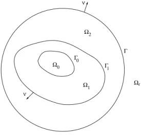
In Section 2.2, we first introduce the nonlinear external transmission problem and then transform it, using the Dirichlet-to-Neumann map, into a boundary value problem in a bounded domain. Thus, using (2.2.9) we lead to a boundary value problem on Ω with an implicit Neumann boundary condition on the circle Γ.
The variational formulations
Additionally, if u|Γ∈[Hm+12(Γ)]2 for some positive integer m, then there exists C >0, independent of N and m, so that the following error estimate holds. For this purpose, we now recall from Lemma 3.3 in [55] that the following estimate holds for all v∈X.
The Galerkin approximations
The error analysis
An example of finite element subspaces
It is well known that Xh and Mh form the simplest Hood and Taylor finite element subspaces satisfying the discrete inf-sup condition (2.4.2) (see e.g. section VI.6 of [20] in the case of equilateral triangles ).
The a-posteriori error estimator
Preliminaries
Here regular means that the interior angles of all the triangles of all the triangles Th are bounded uniformly from below. Thus, in what follows, C will denote a positive constant that may depend on the above uniform bound but not on the mesh size h. Now, for anyT ∈ Th we denote by νT the unit outward normal and by E(T) the set of its edges.
Since {Th}h∈I is a regular family of triangles, it is easy to see that the number of triangles in ∆(T) and in ∆(S) is bounded, independent of h.
Main estimates
Moreover, using the analysis from [29] and [17], we can show that Xhalso satisfies the local properties stated in the following lemma. The involved non-linearity and non-locality of the approximate Dirichlet-Neumann mapping QN actually makes a proper analysis difficult. It is also important to emphasize that a possible a-posteriori analysis of the error ||(u, p)−(uNh, pNh)||X×M should deal with the additional problems caused by the inconsistency of the Galerkin scheme (2.4.1) .
To prove Theorem 2.5.1, we first need some properties for a function depending on the stored energy function Ψ (cf. Therefore, we apply the inequalities to the nonlinear coefficient saij, given by (2.3.9) and ( 2.3.10) , and using Korn's inequality and the continuity of the strain tensor e, we conclude (2.5.2), since the linear operator B therefore satisfies the continuous inf-sup condition (cf. Lemma 2.3.3), Brezzi's theory ([20] ) implies that there exists C0 > 0 such that.
Proof of the main Theorem
The resulting variational formula becomes a twofold saddle point operator equation which, for ease of subsequent analysis, is shown to be equivalent to a nonlinear triple saddle point problem. In this way, a slight generalization of the classical Babuˇka-Brezzi theory is applied to demonstrate the correctness of the continuous and discrete formulations and to derive the corresponding a priori error estimates. The aim of this chapter is to extend the approach and results of [48] to the case of mixed constraints.
In addition, we assume that N induces a strongly monotone and Lipschitz-continuous operator from [L2(Ω)]2×2 in its dual. 3.1.3) where ν is the unit outward normal on ΓN and div denotes the usual divergence operator div acting along each row of the corresponding tensor. A slight extension of the usual Babuˇska-Brezzi theory to this kind of problem is provided in Section 3.3. This extended theory is then applied in Section 3.4 to prove the unique solvability of the continuous formulation.
Finally, throughout this chapter C, signed or unsigned, dashes, tildes, or hats indicate positive constants, independent of the parameters and functions involved, which may have different values on different occurrences.

The dual-mixed variational formulation
Finally, throughout this chapter C, with or without subscripts, bars, tildes or caps, indicate positive constants, independent of the parameters and functions involved, which can take different values at different occurrences. while the equilibrium equation becomes. It is not difficult to realize that, similar to the variational formulation obtained in, also has a twofold saddle point structure. Therefore, to prove that our current formulation (3.2.9) is well-posed, we consider instead an equivalent triple saddle point operator equation, in which that condition naturally arises.
On the other hand, we note that by taking τ =Iandq= 1 in the second equation of (3.2.9) we obtain.
An extension of the Babuˇska-Brezzi theory
We proceed similarly to the proof of Theorem 2.4 in [36] and adapt the analysis of [50] to the present situation. We now proceed similarly to the proof of Theorem 3.2 in [36] and again adapt the analysis of [50] to the present situation. Alternatively, assuming Gˆateaux differentiability of the nonlinear operator A1, one can apply the approach from [42] (see Theorem 3.3 there).
Unique solvability of the continuous formulation
To prove the continuous condition of inf-sup for B1, we now seek to identify the space.
The dual-mixed finite element scheme
In the rest of this section we show that (3.5.2) satisfies the hypotheses of Theorem 3.3.2, which certainly depends on the specific finite element subspaces to be used. 2 At this point we recall that the simplest finite element subspace of [H001/2(ΓN)]2 satisfies the approximation property (AP)ξ. To continue the analysis of the discrete inf-sup condition for B, we now proceed as in [12].
As a consequence of the previous lemmata, we can establish the discrete inf-sup condition for B. 2 Next, we identify the discrete kernel of operatorB, which is necessary to prove the discrete inf-sup condition for B1. We conclude this section with a result on the convergence rate of the finite element scheme (3.5.1).
It follows directly from the estimate of Ce in Theorem 3.5.2 and the usual approximation properties of subspaces of finite elements (see e.g.
The a-posteriori error analysis
Then we define the projection of the remainder with respect to the ordinary inner product h·,·iX of X as the unique element (¯t,σ,¯ p)¯ ∈ X such that. This kind of decomposition is not possible for the expression hτ ν,ξ˜hiΓN that appears in the original definition of the functional J2. On the other hand, the advantage of the a-posteriori error estimate θ, which is certainly reliable but not necessarily quasi-efficient, is that it does not need the exact or any approximate solution of (3.6.5), but a suitable resource function ϕh.
In particular, according to Lemma 3.6.2, one should demand that the local traces of ϕh be as close as possible to the corresponding traces of the exact solution u. Therefore, taking into account the polynomial degrees of the finite element subspaces, we propose the following procedure to choose ϕh. In this chapter we use the fully explicit and reliable a posteriori error estimator from Chapter 3 and define an adaptive algorithm induced by this estimator to calculate the mixed finite element solutions of the nonlinear problem studied there.
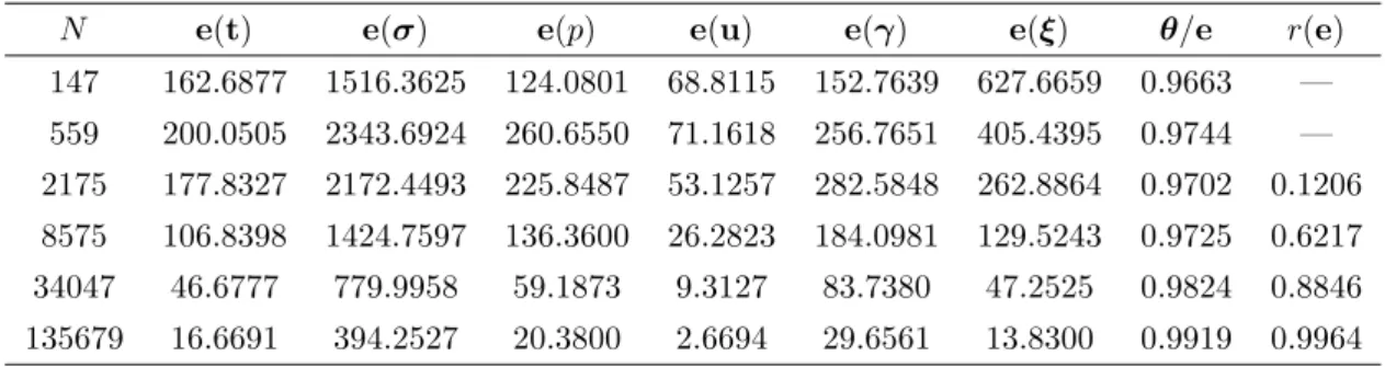
We also recall from Theorem 3.6.3 the completely explicit and reliable a-posteriori error estimate θ of the scheme (3.5.1), given by θ.
Notations and adaptive algorithm
Numerical examples
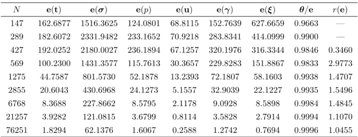
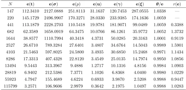
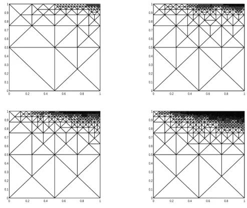
Here we note that u is divergence-free in Ω and has a singular behavior in the outer neighborhood of the segment ]0,1[×{1}. Note that in the pure nonlinear case, the mixed finite element scheme (3.5.1), which becomes a nonlinear algebraic system with N unknowns, is solved by Newton's method with an initial guess given by the solution of the associated linear problem and setting 10−3 as the tolerance for the relative error. We note that this choice works well in each of the examples shown here.
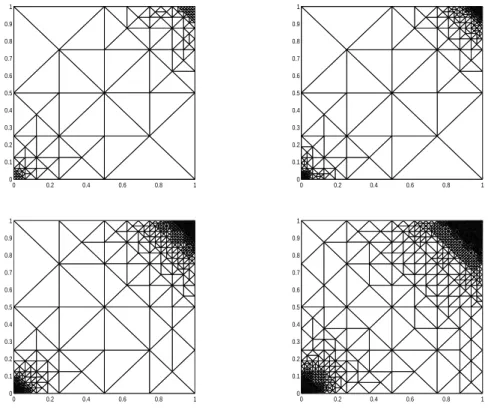
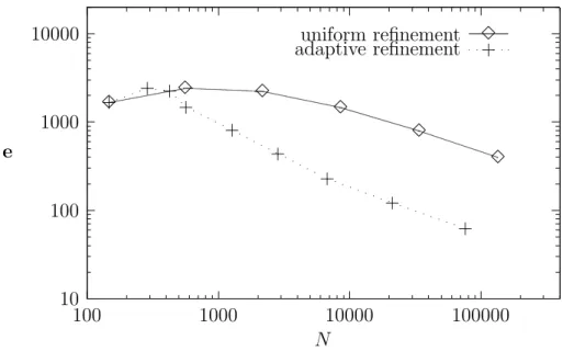
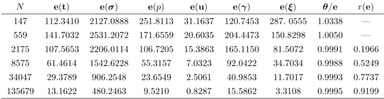
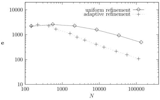
We note that the errors of the adaptive procedure decrease much faster than those obtained by the uniform one. It is also interesting to note that the dominant component of the total error is given bye(σ), which is particularly familiar in Examples 1 and 2. It is interesting to confirm, as expected, that the method is able to recognize all features of the pair solution ( u , p ).
We also note here that the refinement identifies a thin band in an inner neighborhood of the ΓD limit, which corresponds to the flat behavior of the solution caused by the power of 2 in the exponent of the exponential function.
Future work
In: Mathematical Foundations of the Finite Element Method with Applications to Partial Differential Equations, A.K. Stephan, A mixed finite element method for nonlinear elasticity: dual saddle point approach and a- posteriori error estimation. Stein, Symmetric connection of boundary elements and mixed Raviart-Thomas type finite elements in elastostatics.
Funken, A-posteriori error control in low-order finite element discretizations of incompressible steady-state flow problems. Gatica, Combination of Mixed Finite Elements and Dirichlet-to-Neumann Methods in Nonlinear Plane Elasticity. Meddahi, A low-order mixed finite element method for a class of quasi-Newtonian Stokes flows. Part I: a priori error.
Stephan, An implicit-explicit residual error estimator for coupling doubly mixed finite elements and boundary elements in elastostatics.