Je tiens à remercier Dirk Metzler et Jean-Louis Plouhinec avec qui j'ai pu approfondir l'aspect applicatif de ce travail. Merci aux personnes que j'ai rencontrées lors de mon séjour à Orsay et qui m'ont aidé d'une manière ou d'une autre.
L’alignement de s´equences biologiques
M´ethodes d’alignement par programmation dynamique
Une fois qu'une fonction de notation a été choisie (combinaison d'un modèle de substitution et d'une fonction de pénalité d'écart), nous pouvons rechercher l'alignement optimal (celui avec le score le plus élevé). L'algorithme de référence pour l'alignement global de deux séquences est celui de Needleman et Wunsch [62].
Le mod`ele d’´evolution TKF et le mod`ele Markov cach´e pair
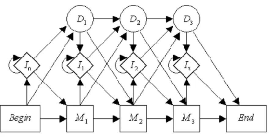
C'est en réponse à ce problème que Bishop et Thompson [9] ont décrit en 1986 une technique pour aligner deux séquences basée sur un modèle évolutif. C'est avec cette définition générale que l'on peut dire que l'alignement sous le modèle TKF est un HMM pair.
Les g´en´eralisations du mod`ele TKF
En fait, la distribution stationnaire des longueurs de séquence selon le modèle TKF91 est (1−λ/µ)(λ/µ)n pour n≥0, ce qui favorise les séquences courtes. La matrice de transition d'alignement dans ce modèle s'écrit comme suit.
L’alignement multiple
Dans ce contexte, l'alignement multiple consiste à mettre des caractères homo dans une même colonne. 1.5 – Chaîne de Markov de l'alignement sous le modèle TKF91 pour un arbre.
Contributions
Un mod`ele d’alignement de s´equences avec des taux d’´evolution
Les zones d'évolution rapide sont divisées en fragments qui évoluent selon le modèle TKF92 avec des paramètres λ < µ (taux d'insertion et de délétion) et γ2 > 1 (taille moyenne des fragments). Les autres paramètres du modèle sont les taux de substitution α1 pour les régions lentes et α2 pour les régions rapides avec α1 < α2.
Estimation param´etrique dans le mod`ele Markov cach´e pair
Nous présentons des applications de notre modèle à des données simulées et réelles. La définition de la probabilité des observations dans le modèle paire-HMM est ambiguë.
Estimation param´etrique dans les mod`eles d’alignement multiple
The parameters of this model are the rates of insertions and deletions and the mean length of the fragments. For the estimation of evolutionary parameters, alignments and segmentations of the sequences, we propose two complementary approaches.
The model
The Insertion and Deletion Process
The new fragment is of type "fast", independent of the type of its ancestor, and its length is geometrically distributed with the expectation γ2. Under these assumptions and with the deletion rate exceeding the insertion rate, the stationary distribution of the number of fast fragments in the stretch is geometric on {0,1,2,.
The Markov property of the alignment
For example, the probability of going from a match in a fast fragment to a slow fragment is the probability that we are on the last fast fragment of the segment, 1− λµ, at the end of this fragment, γ1. Finally, the probability of getting any fast state from the BBS is the probability that the slow fragment terminates, γ1. If this fast state is, for example, BF, this would be the last λβ, the probability that the slow fragment has at least one survivor.
Reversibility of the homology structure
Algorithms
- The likelihood
- ML-estimation of parameters
- MCMC sampling of parameters and alignments
- Alignment sampling
Moreover, the complete distribution (or complete probability) of the observed sequences and an alignment is given by . This is the expression of the complete probability, which we will use in the following. Therefore, one should use some version of the EM algorithm, [18] which maximizes the likelihood of missing data models (we actually observe the sequences but not the alignment).
Applications
Application to simulated data
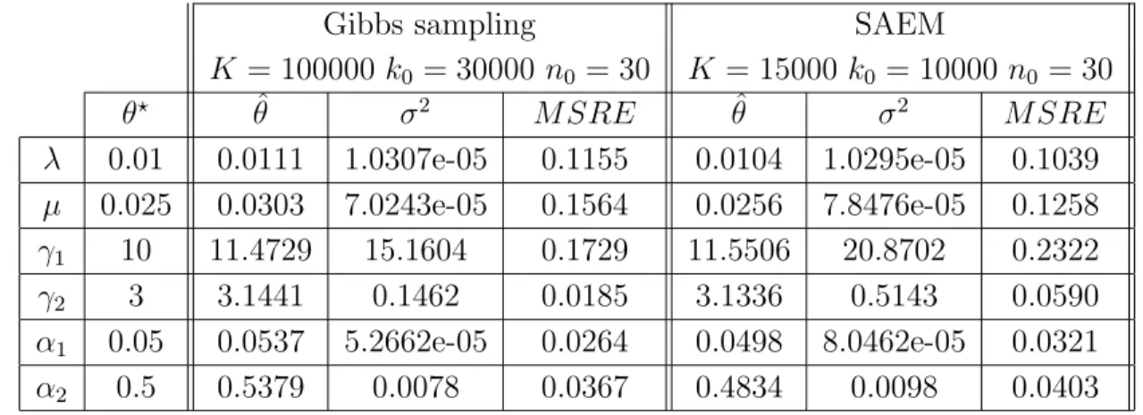
2.1 – Evolution of the iterations of the Gibbs approximation of the posterior means (left) and the SAEM estimator (right) in a single simulation from the first set of parameters. 2.2 – Evolution of iterations of the Gibbs approximation of the posterior means (left) and the SAEM estimator (right) in a single simulation from a different set of parameters. If we are interested in the segmentation of one of the sequences (the first one for example).
Application to real data
Discussion
We intend to generalize our model to the alignment of more than two sequences. In this chapter, we deal with parameter estimation in pairs of hidden Markov models (pair HMMs). The existence of two different levels of information deviation is established and the deviation property is shown under additional assumptions.
Introduction
Background
One of the advantages of the TKF model lies in its exact correspondence with a model containing a hidden Markov structure, which ensures the existence of powerful algorithmic tools based on dynamic programming methods. Observations in a pairwise HMM are formed by a pair of sequences (the ones to be aligned) and the model assumes that the hidden (i.e. unobserved) alignment sequence {εt}t is a Markov chain that determine the probability distribution of the observations. This can be done with MCMC procedures which again require the use of the forward algorithm (Metzler [55]; Arribas-Gilet al.
Roadmap
To examine consistency of estimators obtained by maximization, one needs to understand the asymptotic behavior of the criteria. We adopt the Information Theory terminology and call Information Deviation Rates the difference between the limiting values of the log-likelihoods at the (unknown) true parameter value and at another parameter value. Section 4 then gives the statistical consequences in terms of consistent estimation of the parameters obtained via MLE or Bayesian estimation using pairwise HMM algorithms (see Theorems 3, 4).
The pair hidden Markov model
Model description
Under the hidden random walk condition, the observations are drawn according to the following scheme. Note that a necessary condition for the θ parameter to be recognizable is that the probability of the occurrence of two aligned letters differs from the probability of the product of these letters. Thus, in this case the distribution of observations is independent of the hidden process and the parameter π cannot be identified.
Observations and likelihoods
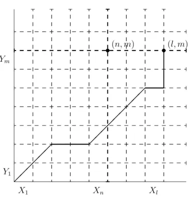
Let us also denote the marginal by hX (resp. hY) with respect to the first (resp. second) coordinate of the distribution h. But since the underlying process {Zt}t≥0 is not observed, the quantity `t(θ) is not a function of the observations alone. In other words, Qθ is the probability of the observed sequences under the assumption that the underlying process {εt}t≥1 passes through the point (n, m).
Biologically motivated restrictions
The aim is to obtain an objective choice of the parameters appearing in the scoring scheme, taking into account the evolution. We thus introduce the following assumption about the stationary distribution of the hidden Markov chain. Assumption of time reversibility in the substitution process implies equality between the marginals of h and individual distributions of the letters, namely hX = f and hY = g.
Information divergence rates
Definition of Information divergence rates
Since the process (εt)t∈N is stationary, we obtain that the distribution (Ws,t) is the same as the distribution (Ws+k,t+k) for any k, so that point 2.
Divergence properties of Information divergence rates
Note that in case assumption 2 holds, the expectations of ε1 under θ and under θ0 are in line with (0,0). To calculate the value of the expectation E0[wt(θ)], set the set At of all possible values of Zt. Now, using easy Cramer-Chernoff bounds, since π is irreducible, one has that there exists a positive c(η) and some s0 >0 as soon as s≥s0,.
Continuity properties
Let μθi, πθi,fθi, gθi and hθi denote the parameters of the hidden Markov chain and emission distributions under θi, i= 1,2.
Statistical properties of estimators
MCMC algorithms approximate the random distribution ν|X1:Nt,Y1:Mt, interpreted as a posterior measure given the observations X1:Nt and Y1:Mt.
Simulations
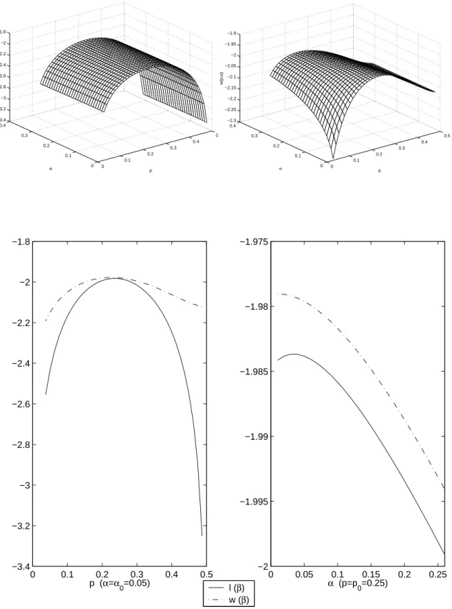
A simple model
We see that both w and ` are very flat with respect to α, and when dealing with numerical precision errors it becomes impossible to find the true maximum value. But for p= p0, if we look closely at the intersections of ` and w, we understand that ` takes its maximum at α0 and w near this point. Regarding p, we see that both ` and w have a clear maximum near p0, but again ` is less flat than w at this point.
Simulations with Markov chains satisfying Assumption 2
3.5 – Histograms of maximum likelihood estimates of parameters obtained with 200 simulations from the Markov chain model. On the left: the estimate of the transition probabilities according to α = α0 and the estimate of α according to the true value of the transition probabilities. In Figure 3.5, we can see that the maximum likelihood estimators for these parameters and for α are close to their true values, even when the estimation is done together.
Discussion
A star tree
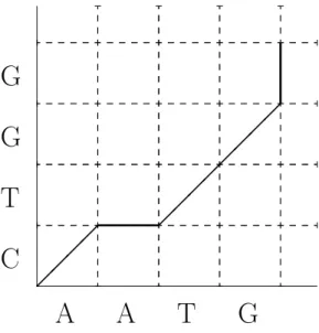
Two charactersXji and Xhl will be aligned in the same column if and only if they are homologous to the same main string character. This is because the Markov dependence for root-leaf pairwise alignments applies independently to each sequence due to the branch independence of the evolutionary process. The homology structure can be described in terms of the nucleotides in the root sequence.
The homology structure model
Model description
When calculating the probability of one pairwise alignment (and the probability of the homology structure is obtained as the sum of the probabilities of several alignments) under TKF91 as the product of the transition probability given in (1.5), there is a factor . It is possible that there are no insertions between two homologous positions in any of the observed sequences. We do not consider branch lengths as parameter components and assume that they are known.
Observations and likelihoods
But since the underlying process {Zn}n≥1 is not observed, the quantity `n(θ) is not a measurable function of the observations. In other words, Qθ is the probability of the observed sequences assuming that the underlying process {εn}n≥1 passes through the point (n1, . . . , nk). It is clear from our definition of homology structure that there is no deterministic relationship between the length of the ancestral sequence and the lengths of the observed sequences.
The case of two sequences
Information divergence rates
Definition of Information divergence rates
Recall that D∗ is what is commonly called the degree of information divergence in information theory: it is the limit of the normalized Kullback-Leibler divergence between the distributions of observations at the true value of the parameter and another value of the parameter. We will use the following version of the subadditive ergodic theorem of Kingman (1968) to prove the points. A similar proof can be written for ii) and is left to the reader. To understand the distribution of (Wm,n)0≤m To calculate the expectation value E0[wn(θ)], consider that the set of all possible values of Zn is Nk. The equilibrium probability distributionν(·) is assumed to be known and will not be part of the parameter. Simulation results Discussion Un mod`ele d’alignement de s´equences avec des taux d’´evolution variables Estimation param´etrique dans les mod`eles d’alignement multiple issusDivergence properties of Information divergence rates
Simulations
The substitution model
L’alignement de s´ equences biologiques