Finite Element Modelling for Materials Engineers Using MATLAB.

(1)

UNIVERSITY OF IBADAN LIBRARY

(2)

Contents

. ^,

1 Introduction '...,...

...

2 ^.^,- .-The ^.,- Weak . _ _ ... Fo~nlAt&n ... ³

...

2.1.. odd ~inite~i'&ents.. : ³

. ... ...

...

. -2.2 - M& ~le&n&j. 3

. . .

...

2.3 The Finite ~lem&t Method ~roceclure. 3 . 214'. Weak Formulation of Governing Equations ... ^;. . . . ⁴

...

2.5 . 'Gradient and Divergence Theorems ⁴

...

.

2.5.1. he ~raciient he or em.. .'. ⁵

...

. , 2 5 2 DivergenceTheorem 5

...

2.6 Integration- by P& .... : ^6.

...

2.7 Weak Forrnulatio'hs : ... ⁶^-

, . -

2.8 EX-~. ... ^=.-.... .- ...-...-.-... If

.-. ... ...

...

Refgences , ^,,,, .. . 12

. ^{. .}

... ...

3 Linear Interpolation ~ c t i o m ^; 13

...

3.1 Parameter Functions and Inte~polating Functions. 13

. . .

3.2 Interpolation, 'Weighting . and Approximation Functions 13

. . .

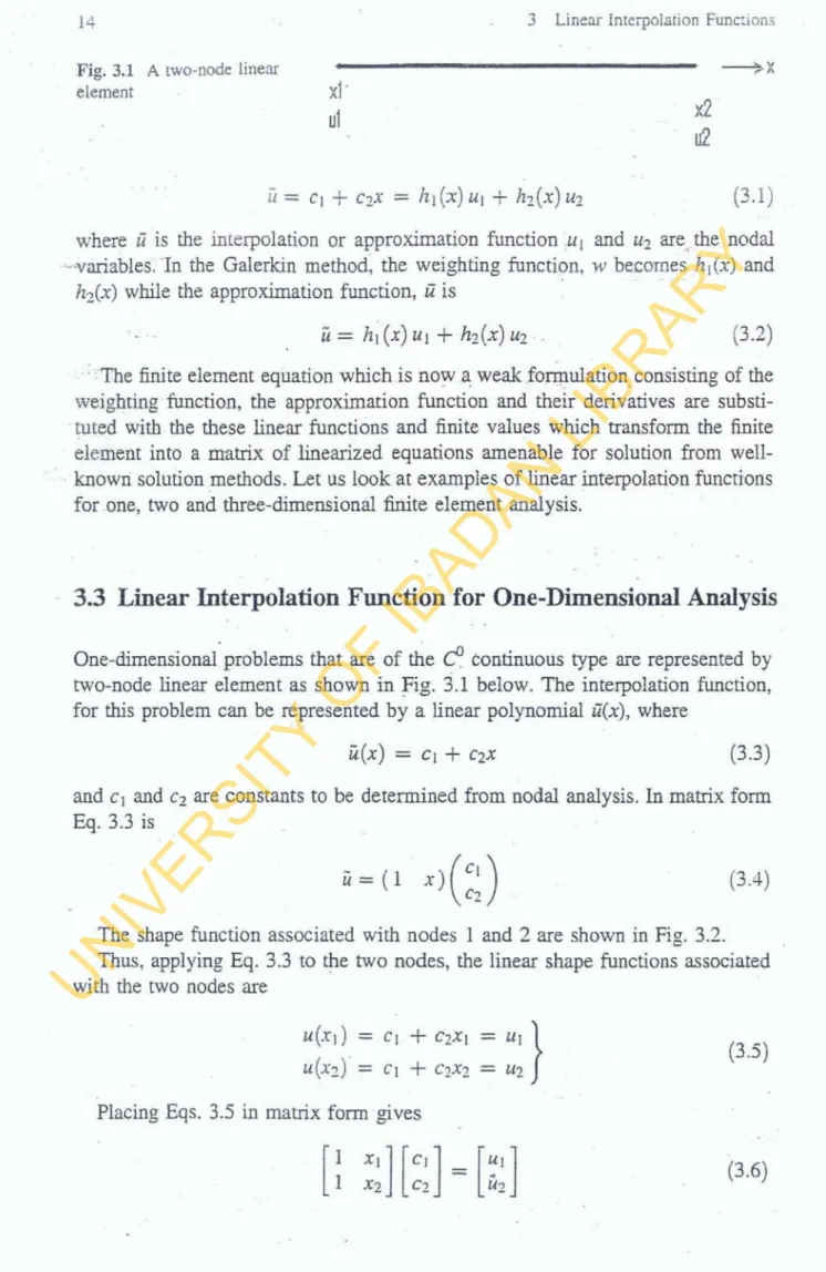
. 3.3 Linear Interpolation Function for One-Dimensional Analysis 14

...

3.4 . Linear Interpolation Functions for Two-Dimensional Analysis 16

...

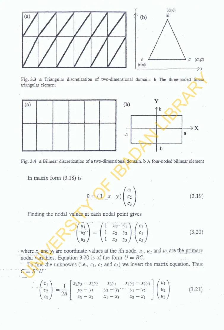
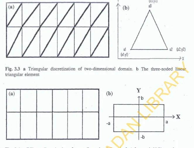
. . 3.4.1 The Linear Triangular Element. 16

3.4.2 The Bilinear Element . . . ¹⁹

3.5 LineaqInterpolation Fll~lctions for

...

. .

.. 'l'&i%-Dheiisionil Problems 21

...

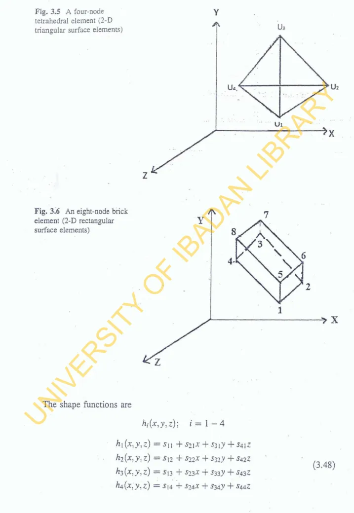
. . . 3.5,..1.-, . Four-Node Tetrahedral Elements. 21

. . ^,

...

. . - 3.5.2 : ^.Eight-Node Brick _Element~,. ^:^, , ²³

3.6. ^'_ :Other.-Coordinate ^... _-. _{. .}_..-..,-. _.:: SystemsUsed in .Denvation ^. ^. ^._- ^.

.*- --

. . . . ..." * - ,"sz.~."-': .... :----;-* . . . a .

...

- - 6 - ^._{..._.} & ... _.-..+ -Y<*ii~.*i .i*. +-.*.. ... ^.>- ^-1:-,.-.+:. 23

: ... . . . -:-fa ^-,,-A*_*^,,,.'_se;;endip1ty _..:: coordinates. ^;.;;-::; ;,..-;., . .::, ^;... ^;^,*. . .

. .. ,.&.. ^~^-_._, ^.. . ] ; e ~ - - e ~ o o ~ ; . . . . . . ... .. ^,. ^,!^:. :--. . . . ... ^: ^: ^, ^,,:. ²³26

. . . .

3-m ^.._.^l_{._.}... _... _- _...- ... - ^.. ^':

- . ^. . . . 26

...

3.6.4-"Volume Coodiques . ^.:: ^. ^. ^. ^;...

1

27

. . . ^{. . . .}

(3)

. .-

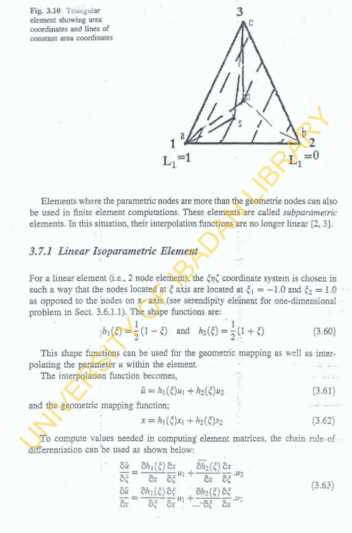
3.7 1% parametric Elements . . . . ^:^:. . . . . . . .. . . . . . . . . . ^{- .}. ^.. . . 27 3.7.1 ^, Linear 1s0'~ararne~tric Element. ^.. . . . ^.... . . . : . . . .' . . 28 3.7'22 ~riangular ~so~arametric Element.. . . . . ; . ^..^.:.. . . -. . . 29 ^.^- 3.7.3 Quadrilateral I s o ~ a r a m e ~ c Element . . . ^.. . . . . . ^.^,^.^;^..^.^, ³¹

3.8 Exercises . . . . . . . . . . . . . . . . . . . . . . . . . . . . . ^{. .}. . . . . 32 References : . . . . . . ^;.. . . . . . . . . . . . . . . ^.. . - . . . . . ^.. . ^-³³

4 Derivation of Element' Matrices, Assembly and Solution ^~.

of the Finite Element Equation. . . . . . . . ^;. . . . . ³⁵

4.. 1 Derivation of Element Matrix for One-Dimensional Problems

Using the Galerkin Method, Assembly and. Solution . . . . . . . ³⁵

4.1.1 Weak Formulation. . . . . . . . . ^{. .}. ^{. . .}. . . . . . . . . . 35 4.1.2 Assembly of Element Equations . . . . . . . . . . . -. . . . . ³⁶

4.1.3 Imposition of Boundary Conditions.. ^{. .}. . . . . . . .. . . . . ^; 38 4.1.4 Obtaining Neumanp Boundary Conditions at X = 0

a n d X = l . . . 39 4.2 Derivation of Element Matrix for Two-Dimensional Problems

Using the Galerkin Method. . . ^.. . . . . . ^.. . ^.. . . . . ^.. 39 4.2.1 Using Triangular Discretization . . . . . . . . 39

. .-:

4.2.2 ^' i Using Bilinear Elements . . . . ^.. . . ⁴¹

4.3 Derivation of Element Matrix for ~hree-~hnensional Problems ^. ^.. ^'

. Using the Galerkin Method. . . . . . . . . . . :; . . . . . . . . . . . ⁴²

4.4 Transient Problems . . . . . . . . . . ^.. . . ^.. 1.. . . . . . . ⁴³

4.4.1 Time Integration Method for 'Transient Problems . . . . . . ⁴⁴

4.5 Derivation of Matrix Equalions for Axisyn'imetric Problems. . . . ⁴⁶

4.6 Sample Solutions on Elements Matrix Coniputation,

Assembly and Solution. . . . . . . . . . . . . . . .:. . . . . . . . . . 49 4.6.1 .Calculating the Column Vector. . . . . . . . . . ⁵⁴

4.7 One-Dimensional Fourth Order ~ i f f e r e n t i 4 : ~ ~ u a t i o n

. ^.

(Beam ⁱBending Roblem) . . . . . . . . . . . . . ^.;, . . . . . . . . . . . , . 55 4.8 T h e ~ i e of Other Coordinate Systems in env vat ion _...

o f Finije Element Equation. . . . . . . .. . . . .;,. -. . . . . 56

. ...

4.8.1 .Len@ Coordinates . . . .. . . . . ^{. . , .}^.:.. . . ^-. . . ⁵⁶

~ ~

4.8.2 Area Coordinates . . . . . . . . . . . . ;:-. . . . . . . . ^{. . .}. . 57 4.8.3 :volume Coordinates . . . . . . . . . . ⁵⁷

,.. .- : :: 58

4.9 Exercises . . . . . . . . . . . . . . . ^+._~.. _.'. . . . . . . . . . . . . . ^.

References .: . . . . . . . . . . , ,: ..-.. _-.^.. . . . . ^{. . .}. ^.. ^..^.,;,^{5 8 - ~}

5 Steps to ~ o d e l i n ~ Using ~ ~ ~ t o o l b f l ~raphics In_terface. . 5 . . ^.^:^.^;^:^-^I^:^- 5 9 . -

. ,

5;l Enginering and Modeling . . . . . . . . .. . . . . . . . . ^1.. ^;^:-⁵⁹^,^,

512 Steps for Modeling with the PDEtoolbox . . . ,. . . . _-. . . . . . . . . I- '.. 59 5.2.1 :Starting the MATLAB PDEtool GUI,'. _,= . . . . . ^{. .}. . . . . . ^60.^;

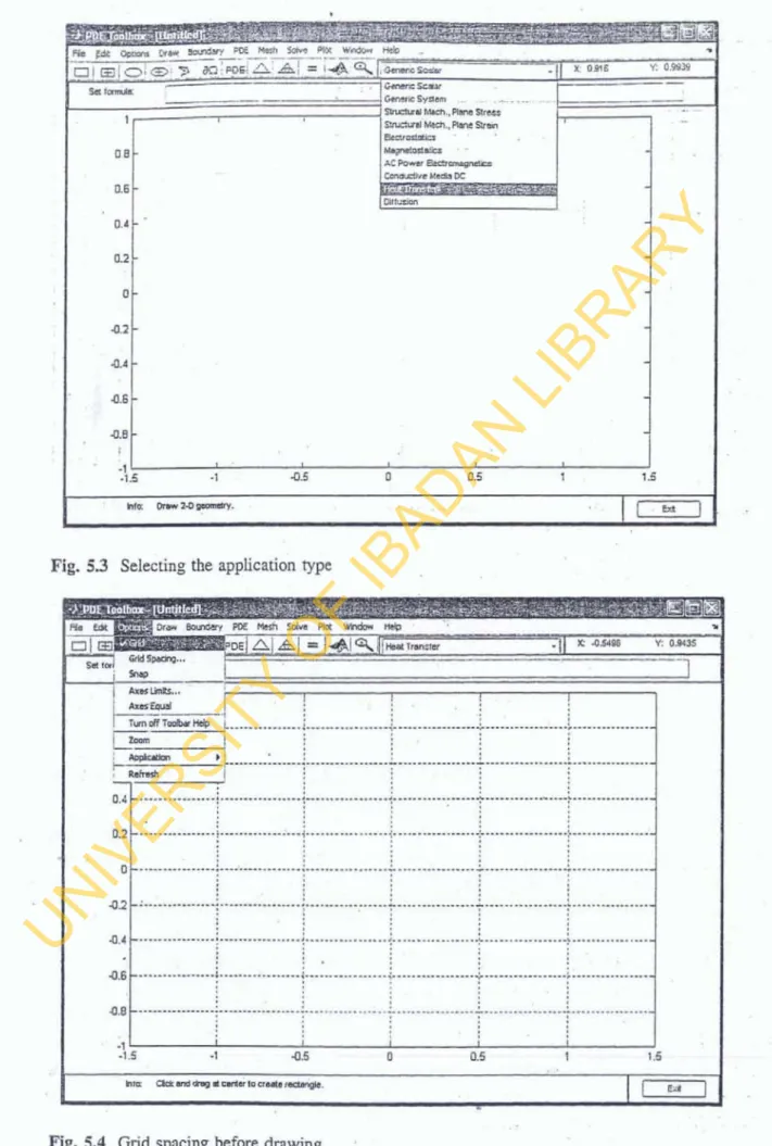
5.2.2 Specifying the Application Type. . . .--. . . . . . . . . . . . . . ⁶⁰^.^.

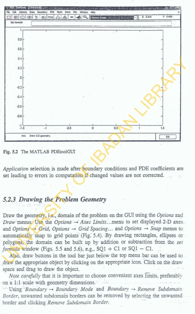
5.2.3 .Drawing the .Problem Geometry . . . .:'. ^,. . . . . ^{. .}. . . . . . 61 ^'.

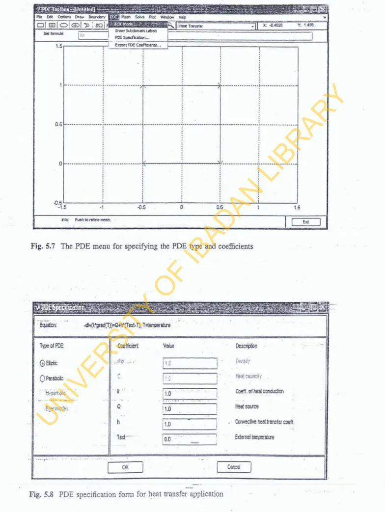
5.2.4 :Specifying the PDE. . . . . . . ; . . . . . _- . . . . ^.. . . 63 ^~ ^.

(4)

...

5.2.5. . Specifying B0urUia.q Cmditions 68

5.2.6 ' mshing the Domain and . Mesh Refinement ... Q

5.2.7 Specifying Initial Conditions for.~ransient Problems . . . . 66

... .

5.2.8 . solving the PDE 66

5.2.9 Expacting Values 'from _Plots. ^;... ⁶⁷

...

5.3 Exercises ^;... ⁷¹

...

References ^'. . . ⁷²

6 Application of toolbox^ ^{to Heat}Transfer Problems ... 73 6.1 Setting-Up the GUI for Heat Transfer Problems . . . ⁷³

6.2 Example Problems on Heat Transfer

. . .

in Materials Engineering 73

...

6.2.1 Steady-State Heat Transfer 74

6.2.2 Transient Problems (Heating and Cooling Problems) . . . 75 6.2.3 Transient Problem (Heat Generation in a

. . .

Tubular Furnace) 80

6.3 Exercises ... ⁸² . . .

References 83

7 Application of P D E ~ O O I ~ O X ~ to Elasticity Problems . . . ^.. 85

. . .

7.1 Basics of Elasticity in Finite Element Application 85 7.2 Using the PDEtoolbox in Modeling Elasticity Problems

. . .

in Materials Engineer@ig 88'

7.3 Applications of PDEtoblbox in Mode* Elasticity Problems .... ⁸⁸. . . . .

7.4 Exe:cises 103

...;... ...

References ., .. ^; ^{. . .}¹⁰⁴

...

'Appendix. -195

(5)

For the Reader-

--.

Note that all the codes in tlie sample problems given in this book _;canbe accessed on htcp://extras.springer.c~rn/. Only some of the codes are pksented in the.

Appendix. There are over25O pages of codes that can easily be copied and pasted on the MATLA.3 M-file irorder to follow'the procedures laid out'in this book. To follow the modeling procedure, the reader can actually copy portiO'ns of the code to be followed on to a new M-file. A new M-file can be opened by1 clicking on 3he

- sheet icon on the MATLAB worksheet. Run the program by clicking on the Debug menu and by double-clicking save and run on the pulldown menu option. This will enable you to follow the solution procedure in an allcolor mode. Other poaions can be added ,as the reader goes along. For example, for the code Diri- c1et.m listed, follow the geometry construction, copy the codes up to the geometry description, and run. Later on to follow boundary conditions, add the codes'for boundary conditions and run again. Then add codes for mesh generation ..., then PDE coefficients, etc until you get to solve the PDE. The reader can follow step by step in this way.

(6)

Chapter 1

~ntroduction

The finite-element method is the solution of variationalfonnulatio of system governing equations applied over a domain discretized into sub-domains (finite elements) with possibility of different boundary conditions on the discretized . surfaces.

Since 'the aim of most analyses is to find unknown functions which satisfy a known set of differential equations in a domain with all sorts of boundary conditions, the finite element method finds useful application in the solution of these problems. Thus, problems solved by the finite element method are either boundary ^' value problems or initial-value problems or both. The solution of most of these .

problems by exact methods of analysis is not possible thereby leaving the option of solution by approximation methods. Thus, it becomes imperative to be able to formulate the problem as a varicrtional problem and to be able toadeive-.$e .- ^- . algebraic equations associated to the variational problem. The least squares,

collocation, Rayleigh-Ritz and the Galerkin methods are wellestablished in solution of many engineering problems and these are well-outlined in mmy books on the finite element method. This book, however, has focused on the use-of the Galerkin method for the solution of the finite-element problems stated &the book.

The use of ~ a t h ~ o r k s ~ pdetoolboxTM presents a faster and efficient tool as it eliminates code writing and post computational analysis.

0. Oluwole, Finite Element Modeling for Materials Engineers Using MATW@, DOI: 10. 1007/978-0-85729461-0-011 (D Springer-Vwlag London Limited 201 1

(7)

(8)

Chapter 2

The Weak ~ o r k l a t i o n

. - ^.^.__,

-..The* nodal Mte methud2s a v a m n a l fomuhion of goycrning equations ap&ed piecewise over' a domain divided into nodal subdivisions. The term'vari-

&al'hne refers to its modem use which permits its use as qpivlent wei&hted integral to the origind problem governing equation (see Sect. 2.4). The principle of solutioii'itself may not necessarily be admissible as a variational priaciple [I].

Clinical treatments of the classical variational formulation terminology can be

assessed in other f o n d texts and handbooks [ 1 4 ] .

Tbe basis of the nodal h i t e element method is the reprcscntation of the domain by an assemblage of subdivisions called bite elements. w e elements are interconnected ^atnodes or nodal points. The trial function appmxjmates the dis- tibution of the ptimary variable m o s s the system of bite elements. Polynomials .

. offer ease of manipulatioL1"and are commonly used'in the nodai ^cipnssim.

3,

2.2 Mesh Elements

Onedimensional (ID) elements are line elements, while 2D elements can be triangular or bilinear elements. Three-dimensional mesh dements are p1yhedrds . or cuboids [7, 81, Distorted elements em also be used [9, 101.

23 The F d t e Element Method Procedure

Same'steps are invalved ⁺ k ⁺ &e 16nik elemem analysis. These ^ape

-- ^{. -.}^"^.

. ^{* .}

-1. I)1M+etlzation of the domix It C R P S ~ of &ection of the shape of mesh

- d d n t s atid .its c o n s d o n . ^-over the whole domain; n u m k h g of the nodes

*and dements and rhe codm@s. ^{. .}

.' - ^. ^' . . . .

,, 2 _,^-:_.L _{I Y .}_.:.,.-,_,-•

: -*L

(9)

2. Select& of interplation kction. .

3. Derivation of v a M o d formlation of the differential equation for a typical element.

4. Derivation of elements stiffness matrix.

5. Assemblage of global stiffness matrix.

6 . Imposition of boundary conditions.

7. Solution of assembled global equation:

8. Representation of results in tabular or graphic form.

2.4 Weak Formulation of Governing Equations

The main approaches of the finite element method are in the redirection of the differential equation of the continuuin problem to its integral form and using a trial function over the nodal form of the equation.

Let us take an approximate trial function as ii = c', hiui where hi is the set of interpolation functions; ^ui is the set of nodal primary variable (displacement, temperature, etc.).

Thus, this function is an approximation solution in the elemental domain defined by a 'set of integral form of the original differential equation.

Thus, a problem in 3D, defined mathematically by a set of differential equations, D valid in a domain R together with the associated boundary condition B can be expressed in a weak formulation as

-

where w is the weighting function and ii is.the trial (approximation) function. The first term in E ~ . 12.1 is further subjected to integratien-by parts.

I . .

. _

' 'Thus, (2.1) is: the approximate form of (2.2)

When wi = hi, the method is the Galerkin method.

2.5 Gradient and Divergence Theorems _-

?,

These theorems are used in the derivation of weak foimulation. Let A and B be scalar functions defined on a 3D domain. UNIVERSITY OF IBADAN LIBRARY-

(10)

2.5.1 The Gradient Theorem

? a - a - a

where V is the gradient operator = ^I- + ^j- + ^k-

ax a,) az 2.5.2 Divergence Theorem

Subsequently from Sects. 2.5.1 and 2.5.2 we can derive the following which are applicable in the inkgation by parts of partial differential equations.

where .. ^..^.^-

a2 a2 a2

v2 ⁼laplacian operator = - + - + -

8x2 ayz az2

and

a a a

V = del operator = pr,G+nyr+n;;-.

, _. . _- _{. . . ,}. . _, _{. , ,} _{. .} oy oz

. . . . .. . . . , .

' 'Ilie'ie text [l 1, 121 will be found _useful.

(11)

2 : The Weak Formulation

2.6- Integration'by Parts

. . .... . . . . . ^. ^. ^{. . .} ^..,.,, ^,, ^,

'If ^k^{i d}^Bare sufficiently differedable I D functions, thei"ihi-f0ll6wing

, . ^.%.,_. . ^{. .}

applicable:

For a first order differential eipiati'oC, ^'

-. ... ^,^,. . ^,,.

or a second order differential equation, _. _.

For a fourth order differential equation,

2.7 Weak Formnlationi ^. ^,

Strong formulation involves evaluation of the highest order of the derivative term in the differential equation. For an example take a 1D second order differential equation d2u/d$ = 0, 0 5 x 5 _{1. In}the weighted residual method, w being the weighting or test function and IZ the approximate solution or the trial function when applied to the equation becomes 1; ^w[d2ii/dx2] dx. Of course d2il/dX2 is the residual of the original differentid equation d2u/dx2. The integral must have a noi-zero finite value to be an approximate solution to the differential equation.

Thus, there is a problem of finding appropriate approximation (trial) function for a strong formulation which must be differentiable in the order of degree of the given differential equation and at the same time has a non-zero finite value.

This problem is removed when integration by parts is applied to the strong formulation reducing it to a weak formulation.

Thus

(12)

2.7 Weak Formulations

-We& formuladons applied over sub domains rkpresent the Finite Element equation. Thus, instead ofidefining ^.~ - trial hnctionin terms of generalized coefficients, the trial function is ::.defined . . in terms of the nodal variables.

.,..

Example 2. I One-dimensiahal, second order differential equations Consider the differential ecuation

. ..Y ..:. . . -

. > , - _,...

. . ddll

subject to the boundary so~ditions - ^u(O)^{= 0}^and^(aa;) ⁼^1.^j

- . -The- weak formulation :~.& be obtained through the following steps. Apply integration by parts (see &it. 2.5.2)

. ^~ ... ~ . .

Equation 2.5 is the weak formulation.

Applying the boundary conditions would give

Equation 2.6 is the weak formulation'with applied boundary condition.

The variational formulation in (2.6) can be expressed as 0 = B(w: u) - ^E(w)

The quadratic functional I (EL) of a variational formulation is represented as

and for the equation under examination this is

. 0

. .

, . *.

. ...

The quadratic fuktio'&l:l(u) represents'. energy in many engineering applica- .tions, the minimization of which gives equilibrium solutipn to the problem. More

. . , . .

(13)

insight in&= use of functionals in finik element analyses can be found in further texts 113-171. It should be noted though, that in a trpical finite element analysis, the domain would be divided into £inite elements each having boundary conditions. In such analysis, the weak formulation that would be applied over the elements will be Eq. 2.5 the limits now being the element dimensions. Thus,

represents the weak formulation of the finite element equation over a domain of n - I 'elements and n nodes.

0-

el'

(-a"'+.)&+ ( w a g )

i=1 d x d x

xi

Example 2.2 Two-dimensional, second order differential equations

XH1

Consider the equation

xi

The weak or variational formulation can be obtained through the following steps:

Weight the integral and obtain the integration by paas of the weighted integral.

Equation 2.8 is the weak formulation to be applied to'thesystem divided into finite elements. This is a typical heat conduction equation. In this case substitute; u:= T. .

If we assume the domain is of rectangular geometry: to be solved as a mono- lithic entity having specified boundary conditions, we can go ahead and substitute the boundary conditions into the weak formulation. ~ s s & n e the boundary condition is convective on one side in the x-direction; (i.e., kaT/ax = -h(T - ^T,))and insulated on the remaining sides (i.e., aT/an = 0 or q = 0).

Then, the boundary integraI $ w(kaT/an) dr becomes

1

Tfre weak formulation in _.. this case will be:

I

k [ b * a ~ awaT) J

o = , -- _ax._ax+--

ay ay ^dw^dy^- ^wh^(T^-^{T ~ )}^dx

R ! r4

(14)

and the quadratic functional

: -

>

Exainple 2.3 Three-dimemiod, second order differential equations Consider the three-dimensional second order PDE.

then the weak formulation over an element @ is derived thus:

Quation (2.10) is the weak formulation.

Example 2.4 Transient problems

Transient problems aie b e dependent or unsteady state problem, Let us consider a ID equation

2 . .. .

The kkak'fomiiiatiori 'is derived &us: ^'^'^,

* Equation 2.1 3 is the weak formulation without applied b o u n w conditio~s.: _{- .}

- h f 7 l e . . 2.5 ^, Fourth or& ~ c r c n t i d equation ^..,. ,

In this ex'mple, it ii 'nec8ssaijr to inregrate by parts ^twiceto distri'bute the

(15)

2 The Weak Formulation.

derivative equation between the dependent variable M and the test function w (also . .

the weighting function) - _.-- ^{. .}^..

for 0 < ^x< L subject to the boundary-conditions

. .,

. .

The weak formulation is derived as follows:

.. . ., , . .

L O = / [ ( . d w ) d ( ' ~ 2 u j -- ^aX.- ^dx^a-^dX2 + y f d x + '] [:'d'(..ii2i)] w- a- ^{. .}^,

d" ^dr2 ⁰ ^.

0

Integrating further gives

This is the weak formulation. Of course when applied to the finite element domain, the integral is taken over the element domain as well as the boundary conditions. Specification of u and du/& i n this equation constitutes the Diriclet or essential boundary conditions and the natural boundary or Neumann conditions are satisfied with the specification of [d/dx(a&)] which is the shear force and

(ad2u/dS) which is the bending moment.

If we apply the boundary conditions, we obtain

A practical example of Example 2.5 is the transverse deflection of a cantilever ,

beam under transverse loading (f) and end moment (Mo). Such an equation will be

, $ [ E I ~ ) + ^f⁼⁰subject to

(16)

2.8 Exercises

Derive the weak fomuMons ^{I &} of he foUowing:

2. Beam under loading force, P

3. For ^atransient heat conduction problem

(17)

1. Reddy JN (2006) An intrOanCrim tq h e dement matbod, 3rd ada PlrlcGraw-Hi&

New Yo&

2 Fi&m BA (1972) me metbod of wightad reaihds Had v&ml prindpIes. Academic

w, ^Hew^York

3. W h i z a K (1975) Variationid methods h elasticity and plasticity. P e r p o n Press.

New Y d

4. Oden ST, W yJN (1983) Vuhfional methods i9 t k m t i d d w , , 2nd edn. w,

New Yo&

5. Reddy JN (2002) 3nergy principles and v a r i a t b d methods in applied mechanics, 2nd cdn.

w&, New Yo&

6. Adnri SN (1987) V m h t i d muple9. In: fidcsmca H, Norrie DH (&I Finite elemcnt bandhok. McOmw-HlI, New Ymk

7, Zienkiewicz OC (1977) The finite element method, 3rd edn. M a w - H i l l , New York 8. Zienkiewiu OC, Morgan K (1983) Flaitee h c n t s md ~ ~ O X McGraw-Hill, E .

NcwYork .

9. Stasa PL (1985) Applicd ^{h i t @}elemmt analysis for enginccrs. CBS Publi- J& Ltd, New Yo& *

10. Ready J?4 .(1986) Applied f m c t i d analysis and v&onal methods, in cngbdng, McGTaw Hill, New Y a k

11. s&& A (1%7) Calclilus and adytic gmmelq. Hole and Winston,New York

12. K q h W (1W3) M vCaICulfl~. ~ MBM~-WCSICY, M a s s a c h m

13. Zidiewich OC, Taylor Rt (1989) The finite dement 'method, Vol. I. M e w - = ,

New York . ^.-

14. H& EM (1975) Tbt fiaite dement metbod f6r ~~. ^W^r^l^e^y^,^New^{Y d}

IS. sathe HJ (1982) b i t e elmat- ^iptpghmhg d y s i s . entice Ha& ~ e w J- 16. Hughes TJR (2000) The finite dement mttbod. b t i c e EM, New Jmcy

17. Z i d k w i c h OC, Taylor RL (1891) Tbe finite eltment &d, Val. 2. M a w - = , ^.

Ncw Yorlc ' ...

(18)

Chapter 3 ^, ^.

Linear Interpolation Functions

3.1 Parameter Functions and Interpolating Functions

'Parameter functions are the now parameters being solved for in problem dehitions. For example, in hcat-tmsfer problem, the nodd parameter is temperature. Thus, parameter functiok are what we refer to as iatqmlation functions (see Sect 3.2) or approximadon functions in the f i n i t e element equation formulation.

These parameter functions need to satisfy two c d t i o n s ; compadbili~ and completeness ^toensure convergence as the domain mesh is refined.

Compatibiliry condition: For ^'^?^t continuous problems, the pantmeter function and its first n derivPtrives must be continuous between elements. Thus in problems in which continuity is d c i e n t , there is no continuity b~tweeq+~elements.

Examples of. continuous p b I e m s are conduction hear transfer where the weak or vari~tional formulation has a h t order derivative (see Examples 2.2 and 2.3).

C' continuous problems are problems that have seeand order derivatives in the we& fornulation such as in beam bending (see Example 2.5 in Chapi,2). ^{. .}.

. Completeness condition: For F continuous problems, the fuoctibn must be able to give a constant value as well as constant partid derivatives up to the (PI + 11th order as ^theelement size decreases to a point For continuou.s -

functions, the parameter function and its first partial. derivdve must give constant

values as the element size decreases to 8 point. An example of a p v e t e r . ^. function fur a continuous _{. .} function is Eq. 3.3 (see Sect. 3.3). L . .'.,. . . . L . ..- . ^.,. . .

If cz is zem, ir = d l . Also, a; d5 = e2. Therefore, the completeness requirement is -

satisfied.

3.2 Interpolation, Weight& and A p p r o ~ t i o n Functions;:

. Znterpolation b t i o n s when mnstnrcted with nodal p h a r y variables . beconie. . . .

approximation fmcZd~ e.g., 9 -

0. OIuwole. Firrite E h m n t ModeIing for Maretiah Ertgineers Using MA-, DO1 ^{: 1}0.1007/97ti-O-85729-66 I -0-5. d Sprinper-Jrer& ^,^. London Limited 201 I