In recent years, the successes of these initial algorithms have led to the use of hierarchical algorithms in many fields. 56] presented the theoretical framework of hierarchical architectures, which enables the study of hierarchical algorithms in practice from a theoretical point of view.
Background and Motivation
Theoretical analysis of hierarchical algorithms can provide insight into the behavior and characteristics of hierarchical architectures. Furthermore, this framework also has the possibility of generalization to include other hierarchical algorithms in practice.
Contributions and Organization of this Paper
Filtering Operations
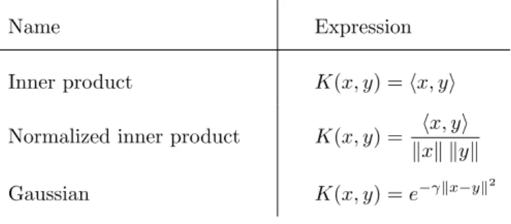
Similarly, Kn is the restriction of K on the subspace(Rn)×n(Rn)⊆`2×`2, and is thus itself a reproducing kernel. Clearly, the normalization of K is equivalent to the condition that the feature map associated with K takes values in the unit sphere in `2, that is, kΦ(x)k = 1 for all x∈ ` 2.
Pooling Functions
Hierarchy of Function Patches and Transformations
For example, the function Ψ(α) =kαk is weakly bounded, while Ψ(α) =kαk2 is not, because we have no upper bound on kαk. Another way to construct function spaces that satisfy Assumption 1 is to start with the function space Im(vn) at the top layer and recursively define the function spaces at lower levels by restricting the functions.
Templates
Otherwise, we say that Tm is a set of templates of the second kind if it is not of the first kind. In particular, when we use templates of the first kind, we start with a set of function patches Tm ⊆ Im(vm) and take the templates to beTm={Nbm(t)|t∈Tm}.
Neural Response and Derived Kernel
The results are then combined into the neural response of the original function. Finally, the kernel function on wm manifests as a linear combination of the kernel functions on the individual components.
Examples of Architectures
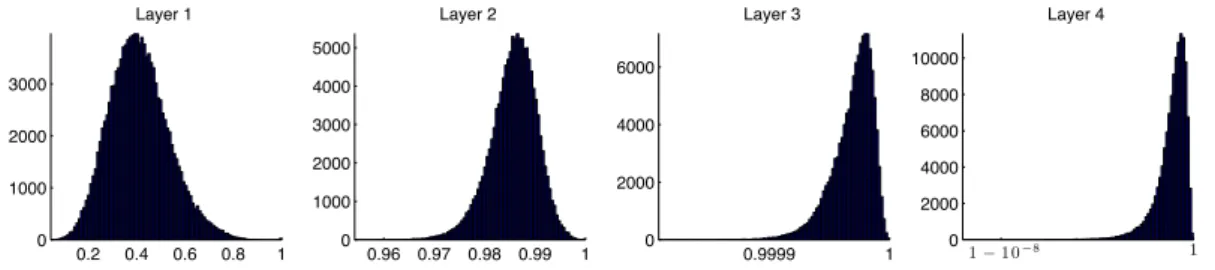
Our approach is to determine a layer-wise lower bound on the compression rate of the derived kernel. In particular, in the case of the 4-layer architecture, we see that the effective volume of the derived core has a width of about 10-8.
Setting and Preliminaries
Nonnegative Architectures
In particular, the histogram for the 1-layer architecture corresponds to the distribution of the normalized inner product between the original images. In particular, we will take the pattern setTm to be a finite set of convex combinations of patterns of the first kind.
Strongly Bounded Pooling Functions
For example, we can restrict the domains of the pool functions in Table 2 to meet this requirement. That is, if Φ:`2→`2 is the feature map corresponding to the kernel function K:`2×`2 → R, then each templateτ ∈ Tmis is of the form.
Dynamic Range of the Derived Kernel
Range Compression: Normalized Kernel Functions
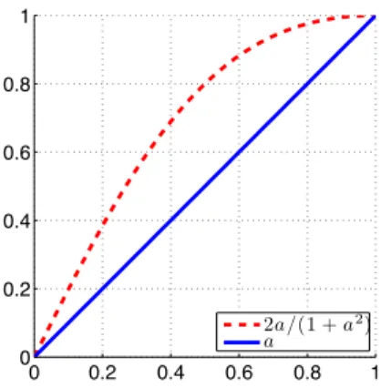
Assume that the feature map Φ corresponding to K is 1- Lipschitz with respect to the normalized metric, . The value 1/2 is obtained by noting that the function we are trying to minimize above ina is decreasing, so its minimum occurs ata= 1, and it is indeed easy to show that the minimum value is 1/2 by ' an application of the L'Hˆospital's rule.
Range Compression: Normalized Pooling Functions
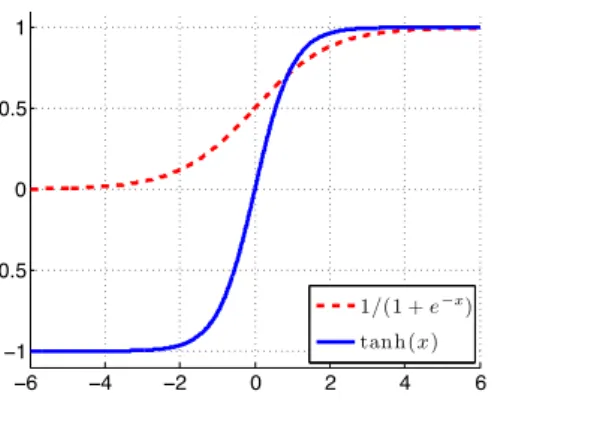
When we work with a non-negative architecture, the presence of the sigmoid function also leads to area compression. Intuitively, this is because the sigmoid function is approximately constant for sufficiently large inputs, which implies that the values of the derivative kernel converge to a stable limit.
Empirical Results and Possible Fixes to Range Compression
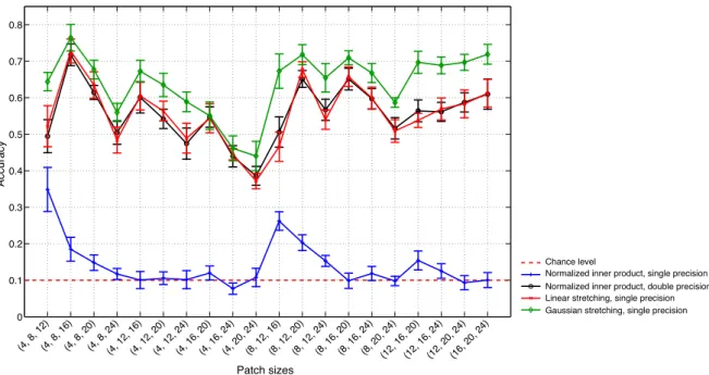
In Figure 4, we see that the accuracy of the normalized inner product kernel with single precision is significantly lower than that with double precision. In fact, the average precision of the single precision normalized inner product kernel is very close to the 1/10 = 0.1 chance level. Apparently, both linear and Gaussian stretching techniques succeed in recovering the dynamic range of the derived kernel.
Both stretching techniques restore the dynamic range of the derived kernel, but Gaussian stretching restores a more symmetric distribution. Moreover, our experiments also confirm that both linear and Gaussian stretching techniques can recover the performance of the four-layer architecture in the environment with some precision.
Discussion
Alinear architecture is a hierarchical architecture with the normalized inner product kernel and a linear pooling function.f For 1≤m≤n, let Nm denote the closed linear span of the neural responses at layerm. We first examine how the choice of the parameters at the first layer limits the complexity of the architecture. We find that in a linear architecture, the dimensionality of the neural response at each layer is limited by the dimensionality of the first layer.
We refer to this phenomenon as therank restriction, which derives from the observation that when the setTmat templates each layer is finite and we merge the templates into Tminto a matrix, then the rank of the matrix is bounded by the rank of the templates matrix at the beginning. lawyer. In the case of a linear architecture, Theorem 4.1 then tells us that all posterior neural response spaces are at most k2-dimensional, for 2≤m≤n, regardless of the number of templates we are using.
Basis Independence
We will also characterize the equivalent derived kernel classes in the case of a discriminative architecture. But in general, in this section we will also use templates of the second type. In this case we have the following explicit characterization of the equivalence classes of the derived kernel.
In our analysis, we shall use the following preliminary result for an architecture with an exhaustive set of templates of the first kind. Consider an architecture with ≥2 layers with an exhaustive set of templates of the first kind at each layer.
Reversal Invariance of the Derived Kernel
- Reversal Invariance from the Initial Kernel
- Reversal Invariance from the Transformations
- Reversal Invariance from the Templates
- Impossibility of Learning Reversal Invariance with Exhaustive Templates
Suppose that the transformation setHn−1 consists of some translations and their reversals, i.e. Hn−1 is of the form In the following result, choosing Tm to be the exhaustive set of templates of the first kind allows us to propagate reversal non-invariance up the hierarchy. As a concrete example of the result above, note that kernelK1 given by (8) is reversal invariant if and only if|v1|= 1.
Consider an architecture withn∈Nlayers, where Hm=Lm is the set of all possible translations and Tm is the set of all possible templates of the first kind. With the choice of the initial kernelK1 given by (8), the derived kernelKn is reversal invariant if and only if|v1|= 1.
Equivalence Classes of the Derived Kernel
In sections and 5.2.3 we saw how we can learn reversal invariance on Kn by choosing the parameters of the architecture appropriately. Similarly, we can try to investigate to what extent the hypotheses of the results are necessary. The answer turns out to be no; This is essentially because the symmetry of the template sets does not adequately capture the idea of reversal invariance.
In fact, we will show that when we take Tm to be the set of all possible templates of the first kind, satisfying the symmetry property we just proposed, the derived kernelKn cannot be inversion invariant unless K1 also inverts -invariant is. One way to interpret this result is to say that the templates contribute to the discrimination power of the architecture.
Mirror Symmetry in Two-Dimensional Images
However, when |v1| is sufficiently large, the periodic patterns separate into distinct equivalence classes that we can identify explicitly. The staggered periodic patterns in the equivalence classes of Kn can be interpreted as the translation invariance one hopes to achieve from the pooling operations in the hierarchy, and the periodicity of the patterns emerges because we are working with finite function patches. We assume that the feature spaces consist of all possible images of appropriate size, .
If we think of the first and second coordinates of each patch as the xandy axis, we now define the analogue of the reverse operation on the images, which is the reflection about the axis of them. We can show that the result of Statement 5.14 extends naturally to the case of reflection symmetry.
Discussion
This viewpoint should allow us to extend some of the results in this section to the case of images. In the case of a linear architecture, we have proven that the dimensionality of the neural response at each layer is limited by the dimensionality at the first layer. Moreover, we have shown that when we use an orthonormal basis of the neural responses as templates, the derivative.
Finally, we characterized the equivalence classes of the derived kernel in the case of a discriminative architecture. We believe that a theoretical analysis on the effect of the number of layers in the architecture can provide some insight into this problem.
Strongly Bounded Pooling Functions
Dynamic Range of the Derived Kernel
Since we are holding everything fixed except ω1, we can only consider cosθ as a function of ω1. Since dcosθ/dω1>0 forω1< AD/B andcosθ/dω1<0 forω1> AD/B we conclude that ω1=AD/B is a maximum point of cosθ, as desired. This is because if one of the points, say x0, is not a vertex, it has a coordinate xi such that a < xi < b.
This corresponds to choosing γ = δ = 0, in which case the right-hand side of the above inequality becomes 2ab/(a2+b2). Finally, the following lemma relates the dynamic range of the kernel obtained in each layer to the normalized inner product between the neural responses in the next layer.
Range Compression: Normalized Kernel Functions
Range Compression: Normalized Pooling Functions
We note that the assumption thatσ is nondecreasing and concave onR0 is necessary to completeLemma B.4. To see this, suppose we do not assume that σ is non-decreasing or concave, so that σ0 need not be non-negative and non-increasing. wherebxcis is the largest integer less than or equal to tox. Next, suppose we assume that σ is non-decreasing, but we do not assume that σ is concave.
Therefore, the hard limit of Ψ gives us. gOr takeσ0 to be a continuous approximation of the function proposed above. hOr, as before, we can take σ0 to be a continuous approximation of the proposed function. Since Nbm(f◦hi)∈ Nmandτ∈ Tm⊆ Nm, we can expand the inner product in terms of the following orthonormal basis of Nmas,.
Basis Independence
The above calculation shows that for each f ∈Im(vm+1) we can write Nm+1(f) as a linear combination {ϕ1,. Since K is the normalized kernel of the inner product, this implies that the neural responses Nm(f) and Nm(g) are collinear, i.e. Nm(f) = cNm(g) for some c ≥ 0.
Reversal Invariance of the Derived Kernel
- Reversal Invariance from the Initial Kernel
- Reversal Invariance from the Transformations
- Reversal Invariance from the Templates
- Impossibility of Learning Reversal Invariance with Exhaustive Templates
By inspecting the above proof, we see that Theorem 5.6 also holds if we use a general polar function Ψ that is invariant under permutations of its input. We will show that if Km is not reversal invariant, then Km+1 is also not reversal invariant, for 1 ≤ m ≤ n−1. This will imply that if K1 is not reversal invariant, then Kn is also not reversal invariant, as desired.
However, notice that since λ(f)≤ |vm|and each iteration of this process through case (b) increases λ(f), we must eventually land on case (a), in which case we are done, as the failure witness Km+1 to be a plant invariant. Having proved that the reversal Kmis is symmetric for 1≤m≤n, we will now follow the general method of case (1) to show that Kn is not an invariant reversal.
Equivalence Classes of the Derived Kernel
That is, de1 is the smallest d∈N so that we have jumped from j(0) toj(d) times to the right, not necessarily consecutively. Note that such an ade1 must exist, since we cannot jump to the left all the time. Ifde1 De1 >de2, then when we reach j(de2) we would have jumped to the left y times and to the rightre2−y < xtimes. This means fraj(de2), the nextx+y−de2 moves must be jumps to the right, and thus. Neocognitron: A self-organizing neural network model for a position-invariant pattern recognition mechanism.Mirror Symmetry in Two-Dimensional Images