Kriging prediction for manifold-valued random fields

Kriging prediction for manifold-valued random fields

Davide Pigoli^a,∗, Alessandra Menafoglio^b, Piercesare Secchi^b

aStatistical Laboratory, Department of Pure Mathematics and Mathematical Statistics, University of Cambridge, UK

bMOX-Department of Mathematics, Politecnico di Milano, Milan, Italy

Abstract

The statistical analysis of data belonging to Riemannian manifolds is becoming increasingly important in many applications, such as shape analysis, diffusion tensor imaging and the analysis of covariance matrices. In many cases, data are spatially distributed but it is not trivial to take into account spatial dependence in the analysis because of the non linear geometry of the manifold. This work proposes a solution to the problem of spatial prediction for manifold valued data, with a particular focus on the case of positive definite symmetric matrices. Un- der the hypothesis that the dispersion of the observations on the manifold is not too large, data can be projected on a suitably chosen tangent space, where an ad- ditive model can be used to describe the relationship between response variable and covariates. Thus, we generalize classical kriging prediction, dealing with the spatial dependence in this tangent space, where well established Euclidean meth- ods can be used. The proposed kriging prediction is applied to the matrix field of covariances between temperature and precipitation in Quebec, Canada.

Keywords: Non Euclidean data, Residual kriging, Positive definite symmetric matrices

Introduction

This work is part of a line of research which deals with the statistical analysis of data belonging to Riemannian manifolds. Studies in this field have been mo- tivated by many applications: for example Shape Analysis (see, e.g, Jung et al., 2011), Diffusion Tensor Imaging (see Dryden et al., 2009, and references therein)

∗Corresponding address: Statistical Laboratory, Centre for Mathematical Sciences, Wilber- force Road, Cambridge CB3 0WB, United Kingdom. Email address: [email protected]

and estimation of covariance structures (Pigoli et al., 2014). Using the termi- nology of Object Oriented Data Analysis (Wang and Marron, 2007), in all these applications the atom of the statistical analysis belongs to a Riemannian mani- fold and therefore its geometrical properties should be taken into account in the statistical analysis.

We develop here a kriging procedure for Riemannian data. Spatial statistics for complex data has recently received much attention within the field of functional data analysis (see Nerini et al., 2010; Delicado et al., 2012; Gromenko et al., 2012;

Menafoglio et al., 2013, 2014; Menafoglio and Petris, 2015) but the extension to non Euclidean data is even a greater challenge because they do not belong to a vector space.

Many works have considered the problem of dealing with manifold-valued response variables. Some of them propose non parametric (see Yuan et al., 2012, and references therein) or semi-parametric (see Shi et al., 2012) approaches but this implies a lack of interpretability or the reduction of multivariate predictors to univariate features. In particular, these approaches do not allow to introduce the spatial information in the prediction procedure.

A different line of research is followed in the present work, along the lines of those who try to extend to manifold-valued data parametric (generalized) lin- ear models (see, e.g. Fletcher, 2013). We propose a linear regression model for Riemannian data based on a tangent space approximation. Even though the lat- ter model is here developed in view of kriging prediction for manifold data, it may be used in general to address parametric regression in the context of Rieman- nian data, since it allows to consider multiple predictors in models with manifold- valued response variables. The central idea of this work consists in using the local geometry of the manifold to find a data-driven linearization, i.e. looking for the tangent space where the parametric model provides the best possible fitting for the available data.

The proposed method is illustrated here for the special case of positive definite symmetric matrices and in view of a meteorological application to covariance matrices. More in general, this approach is valid every time a Hilbert tangent space and correspondent logarithmic and exponential map can be defined, as we show in the Appendix.

1. Statistical analysis of positive definite symmetric matrices

Positive definite symmetric matrices are an important instance of data belong- ing to a Riemannian manifold. In this section, we introduce notation and a few

metrics, together with their properties, that we deem useful when dealing with data that are positive definite symmetric matrices. A broad introduction to the statistical analysis of this kind of data can be found, e.g., in Pennec et al. (2006) or Dryden et al. (2009).

LetP D(p)indicate the Riemannian manifold of positive definite symmetric matrices of dimension p. It is a convex subset of R^p(p+1)/2 but it is not a linear space: in general, a linear combination of elements ofP D(p)does not belong to P D(p). Moreover, the Euclidean distance inR^p(p+1)/2 is not suitable to compare positive definite symmetric matrices (see Moakher, 2005, for details). Thus, more appropriate metrics need to be used for statistical analysis. A good choice could be a Riemannian distance: the shortest path between two points on a manifold, once this has been equipped with a Riemannian metric, as we illustrate below. A description of the properties of Riemannian manifolds in general, and of P D(p) in particular, can be found in Moakher and Z´era¨ı (2011) and references therein.

LetSym(p)be the space of symmetric matrices of dimensionp. The tangent spaceT_ΣP D(p)to the manifold of positive definite symmetric matrices of dimen- sionpin the pointΣ∈P D(p)can be identified with the spaceSym(p), which is linear and can be equipped with an inner product. A Riemannian metric inP D(p) is then induced by the inner product in Sym(p). Indeed, the choice of the inner product in the tangent space determines the form of the geodesic (i.e. the short- est path between two elements on the manifold) and thus the expression of the geodesic distance between two positive definite symmetric matrices. A possible choice for the Riemannian metric is generated by the scaled Frobenius inner prod- uct in Sym(p), which is defined as⟨A, B⟩Σ = trace(Σ⁻¹²A^TΣ⁻¹BΣ⁻¹²), where A, B ∈ Sym(p). This choice is very popular for covariance matrices, because it generates a distance which is invariant under affine transformation of the random variables.

For every pair(Σ, A) ∈ P D(p)×Sym(p), there is a unique geodesic curve g(t)such that

g(0) = Σ, g^′(0) =A.

When the Riemannian metric is generated by the scaled Frobenius inner product, the expression of the geodesic becomes

g(t) = Σ¹² exp(tΣ⁻¹²AΣ⁻¹²)Σ¹²,

whereexp(C)indicates the exponential matrix ofC ∈Sym(p). The exponential

map ofP D(p)inΣis defined as the point att= 1of this geodesic:

exp_Σ(A) = Σ¹² exp(Σ⁻¹²AΣ⁻¹²)Σ¹².

Thus, the exponential map takes the geodesic passing throughΣwith “direction”

Aand follows it untilt = 1. The exponential map has an inverse which is called logarithmic map and is defined as

log_Σ(P) = Σ¹² log(Σ⁻¹²PΣ⁻¹²)Σ¹²,

where log(D) is the logarithmic matrix of D ∈ P D(p). The logarithmic map returns the tangent elementAthat allows the corresponding geodesic to reachP att= 1.

TheRiemannian distancebetween elementsP1, P2 ∈ P D(p)is the length of the geodesic connectingP₁ andP₂, i.e.

d_R(P₁, P₂) = ||log(P₁^−1/2P₂P₁^−1/2)||F = vu ut∑^p

i=1

(logr_i)²,

where the r_i are the eigenvalues of the matrixP₁⁻¹P₂ and ||.||F is the Frobenius norm for matrices, defined as

||A||F =√

trace(A^TA).

This distance is called affine invariant Riemannian metric or trace metric, for instance in Yuan et al. (2012).

Other distances have been proposed in the literature to compare two positive definite symmetric matrices, both for computational reasons (Pennec et al., 2006) and for convenience in specific problems (Dryden et al., 2009). For example, we may consider the Cholesky decomposition of the positive definite symmetric matrixP, i.e. the lower triangular matrix with positive entriesL= chol(P)such that P = LL^T. Then, Wang et al. (2004) defined a Cholesky distance between two positive definite symmetric matrices as

d_C(P₁, P₂) =||chol(P₁)−chol(P₂)||F, while Pennec (2006) proposed the Log-Euclidean distance

d_L(P₁, P₂) =||log(P₁)−log(P₂)||F,

based on the matrix logarithm. Another possibility is to resort to the square root distance(Dryden et al., 2009):

d_S(P₁, P₂) = ||P

1 2

1 −P

1 2

2 ||F,

whereP¹² is the matrix square root ofP. It is worth to notice that the square root distance is also defined for non negative definite matrices. Thus, it is to be pre- ferred in applications where matrix data may have zero eigenvalues, or very small eigenvalues which lead to instability in the computation of the affine invariant Riemannian distance, the Cholesky decomposition or the matrix logarithm.

Each definition of distance has a corresponding geodesic and thus exponential and logarithmic map. For example, the geodesic curve associated with the square root metric inΣ∈P D(p)with tangent vectorA ∈Sym(p)is

g(t) = (Σ¹² +tA)^T(Σ¹² +tA), t≥0,

and the corresponding exponential and logarithmic map are therefore exp_Σ(A) = (Σ¹² +A)^T(Σ¹² +A),

log_Σ(P) =P¹² −Σ¹².

The expression of the logarithmic map for the Cholesky and logarithmic distance is similar, the square root transformation being substituted bychol(Σ)andlog(Σ) respectively.

Once a metricd has been introduced inP D(p),we can address the problem of estimating the mean given a sample of positive definite symmetric matrices.

In recent years, many authors (Fletcher et al., 2004; Pennec et al., 2006; Dryden et al., 2009) proposed to use the Fr´echet mean for a more coherent approach in dealing with data belonging to a Riemannian manifold. Note that the Fr´echet mean with respect to a Riemannian distance is often called intrinsic mean in the literature (see, e.g., Bhattacharya and Patrangenaru, 2003, 2005). The Fr´echet mean of a random element S, with probability distribution µ on a Riemannian manifoldM, is defined as

M = arginf

P∈M

∫

d(S, P)²µ(dS) and it can be estimated with the sample Fr´echet mean

S = arginf

P∈M

∑n i=1

d(S_i, P)²,

if (S₁, ..., S_n) is a sample fromµ. In case M = P D(p), both the Fr´echet mean and the sample Fr´echet mean exist and are unique (see, e.g, Osborne et al., 2013, and reference therein). Analogously, the variance ofScan be defined as

σ² = Var(S) =E[d(S, M)²] and estimated with the sample variance

b σ² = 1

n

∑n i=1

d(S_i, S)².

By means of extensive comparisons, Dryden et al. (2009) show that using es- timators based on a Riemannian distance gives better results than the estimator based on Euclidean metric. In particular, the affine-invariant Riemannian metric dR has desirable properties such as avoiding theswelling effect (i.e. the fact that the average has larger determinants than the observation) and providing positive definite matrices also when extrapolating. For these reasons, we are going to pre- fer the affine-invariant Riemannian metric for the application of the Kriging pro- cedure. However, these advantages come with a relevant computational cost that may be too heavy in some applications, for example in Diffusion Tensor Imaging (DTI). The Cholesky distancedC and the Log-Euclidean distancedLprovide then more efficient alternatives. In particular, the Log-Euclidean distance shares most of the good properties of the affine-invariant Riemannian distance (see Pennec et al., 2006, for more details) with the main difference being in producing more anisotropic estimates. Finally, when data can include also non-negative definite matrices, we need to use the square root distanced_S or some of its generalization such as the power Euclidean distance or the Procrustes size-and-shape distance (see Dryden et al., 2009).

In the following, we will need to endow the linear spaceSym(p)of symmetric matrices with a metric; we will consider the metric induced by the Frobenius inner product ⟨·,·⟩F. Based on this, we define the covariance between two random matricesA, B ∈Sym(p)asCov(A, B) = E[⟨A−E[A], B−E[B]⟩F].

Finally, we need some notation for dealing with array of matrices, being these our data. Let T ∈ Sym(p)ⁿ a p×p×n array, where T_..i ∈ Sym(p) for i = 1, . . . , n. Then, we can define a norm for this array as||T||²_Sym(p)ⁿ =∑n

i=1||T_..i||²_F and a scalar product⟨T,U⟩Sym(p)ⁿ = ∑n

i=1⟨T..i, U..i⟩F. Let us consider a matrix G ∈ Sym(n), the product of this matrix for an array T ∈ Sym(p)ⁿ can be defined asGT∈ Sym(p)ⁿ, where(GT)_..i =∑

jG_ijT_..j. A property we need in

the following is that

⟨GT,U⟩Sym(p)ⁿ =⟨T, GU⟩Sym(p)ⁿ,

because of the symmetry of G. Finally, we define the covariance matrix for an array T ∈ Sym(p)ⁿ as the matrixCov(T) ∈ Sym(n) such that [Cov(T)]ij = Cov(T_..i, T_..j).

2. A tangent space model for Riemannian data

Under the hypothesis that the dispersion of the observations on the manifold is not too large, a tangent space can be used to approximate data in a linear space, where an additive model can be employed to describe the relationship between response variable and covariates. This allows to extend well established statis- tical methods for regression models to the context of manifold valued response variable. Let us consider the model

S(x;β,Σ) = exp_Σ(A(x;β) + ∆) (1) whereΣ ∈ P D(p)andA(x;β) ∈ Sym(p)depends on the parameters collected in the array of matricesβ = (β..0, ..., β..r) ∈Sym(p)^r+1, ris the number of pre- dictors andx ∈ R^r is the vector of covariates. ∆ ∈ Sym(p)is a random matrix such that its mean is the null matrix andVar(∆) = σ². Thus, this manifold val- ued random variable is generated following the geodesic passing through Σwith tangent vectorA(x;β) + ∆: the geodesic to be followed to obtain the realization of the variable is controlled by the covariate vector xbut an additive error is also present. The model for the symmetric matrix A has to be specified and in this work we deal with the linear model

A(x;β) =

∑r k=0

β_kZ_k, (2)

where the Z_k’s are the components of the vector Z = (1 x^T)^T ∈ R^r+1. This strategy, involving a tangent space projection, can be followed also to generalize to manifold valued response variables more complex models, such as non linear or generalized regression models. This model follows the general idea proposed in Fletcher (2013) in using the local Euclidean properties of the manifold to define a regression model. The model we propose differs in the fact that the errors are defined in a common tangent space, thus allowing for the extension to the case

of correlated errors we consider in Section 3. Moreover, we use a more flexible model for the symmetric matrix A and this is helpful when modeling the drift effect.

Let us consider a sample((x₁, S₁), . . . ,(x_n, S_n))from model (1) with uncor- related errors. The goal is to fit a tangent plane approximation which best models the relationship betweenxandS, i.e. to find

(Σ,b β) =b argmin

Σ∈P D(p),β∈Sym(p)^r+1

∑n i=1

||

∑r k=0

β_..kZ_ik−log_Σ(S_i)||²F, (3) wherelog_Σ indicates the logarithmic map, which is the inverse of the exponential map and projects each element of P D(p)on the tangent space of P D(p) in Σ, Z = [Z_ik] is then ×(r + 1) design matrix andβ ∈ Sym(p)^r+1 is the array of matrix coefficients. Thus, our estimator looks for the linear model in the tangent space which minimizes the error sum of squares.

For a given knownΣ, minimization of (3) is an ordinary least square problem in the tangent space, since

∑n i=1

||

∑r k=0

β_..kZ_ik−log_Σ(S_i)||²F =

∑n i=1

∑p l=1

∑p q=1

(

∑r k=0

β_lqkZ_ik−(log_Σ(S_i))_lq)² =

=

∑p l=1

∑p q=1

||Zβ_lq.−Y_lq(Σ)||²_Rⁿ,

whereY_lq(Σ)∈Rⁿis the vector((log_Σ(S₁))_lq, . . . ,(log_Σ(S_n))_lq)^T of elements in position(l, q)of the projected observations. Thus, each term of the previous sum is minimized with respect toβ’s by the ordinary least square solution

βb_lq.(Σ) = (Z^TZ)⁻¹Z^TY_lq(Σ), (4) and βb_..k(Σ) ∈ Sym(p) is the estimate for the k-th matrix parameter β_..k. The global solution should thus be in the form(Σ,β(Σ))b and the problem

min

Σ∈P D(p)

∑n i=1

||

∑r k=0

βb_..k(Σ)Z_ik−log_Σ(S_i)||²_F (5)

has to be numerically solved. Here we resort to Nelder-Mead algorithm imple- mented in theoptim()function in the R software (R Development Core Team,

2009), with constraints to ensure the matrix to be positive definite. This works well for two or three dimensional matrices, while in case of higher dimensional matrices more efficient optimization tools would be needed, for example gradient descend or Newton methods on the manifold (see, e.g, Dedieu et al., 2003). In this way, we obtain an estimate for the parameters:









Σ = argminb

Σ∈P D(p)

∑_n

i=1||∑_r

k=0βb_..k(Σ)Z_ik−log_Σ(S_i)||²F, βb_lq.= (Z^TZ)⁻¹Z^TY_lq(Σ)b for 1≤l≤p,1≤q ≤p

(6)

This method asks to specify the model (2) for the matrixA. Since this model is defined on the tangent space, well established techniques can be used for model selection, for example cross-validation.

3. Kriging prediction

In this section we apply the tangent space regression described above to non- stationary manifold-valued random fields. The main idea is to use a tangent space model to approximate the geometry of the manifold and to refer to the tangent space to deal with spatial dependence. Thus, the proposed model is the following:

fors∈D⊂R^d,

S(s;β,Σ) = exp_Σ(A(x(s);β) + ∆(s)), (7) where ∆is a zero-mean, globally second-order stationary and isotropic random field taking values inSym(p), the Euclidean space of symmetric matrices of order p. This means thatE[∆(s)]is the null matrix for allsinDand, fors_i,s_j ∈D, the covariance between∆(si)and∆(sj)depends only on the distance betweensiand s_j, i.e.,Cov(∆(s_i),∆(s_j)) = C(||s_i −s_j||). This definition of the covariogram Cfollows the approach detailed in (Menafoglio et al., 2013) for data belonging to Hilbert spaces. Equivalently, under the previous assumptions, forsi,sj ∈D, the spatial dependence of the field can be represented by the semivariogram defined as γ(||s_i−s_j||) = ¹₂Var(∆(s_i)−∆(s_j)) = ¹₂E[||∆(s_i)−∆(s_j)||²_F].The assumption of isotropy can be relaxed but it brings additional complication in the estimation of the spatial dependence and this is outside of the scope of this work.

Lets₁, ...,s_n be distinct locations in the domainD and assume that, in each location si, the covariate vector x(si) is observed together with a realizationSi

of the random field (7). If the spatial dependence structure was known, the pa- rameters of (7) could be estimated following a generalized least square approach.

Indeed, letΓbe the covariance matrix of the random errors in the observed loca- tions, i.e. Γ_ij =C(||s_i−s_j||)andR∈ Sym(p)ⁿthe array of matrices such that R..i = ∑_r

k=0β..kZik −log_Σ(Si). Thus, Γ^−1/2R ∈ Sym(p)ⁿ has zero mean and identity covariance matrix, since

[Cov(Γ^−1/2R)]_ij =E[⟨(Γ^−1/2R)_..i,(Γ^−1/2R)_..j⟩F] =

=E[⟨∑

l

Γ⁻_il^1/2R_..l,∑

m

Γ⁻_jm^1/2R_..m⟩F] =

=E[∑

l

∑

m

Γ⁻_il^1/2Γ⁻_jm^1/2⟨R_..l, R_..m⟩F] =

=∑

l

∑

m

Γ⁻_il^1/2Γ⁻_jm^1/2E[⟨R..l, R..m⟩F] =

=∑

l

∑

m

Γ⁻_il^1/2Γ⁻_jm^1/2Γ_lm = (Γ^−1/2ΓΓ^−1/2)_ij =

{ 0 i̸=j 1 i=j , whereΓ^−1/2 is the inverse of the matrix square root of Γ. Hence, the generalized least square problem is

(Σ,b β) =b argmin

Σ∈P D(p),β∈Sym(p)^r+1

∑n i=1

||(Γ^−1/2R)_..i||²F = (8)

= argmin

Σ,β

∑

i

∑

j

(Γ⁻¹)_ij⟨

∑r k=0

β_..k(Σ)Z_ik−log_Σ(S_i),

∑r k=0

β_..k(Σ)Z_jk−log_Σ(S_j)⟩F. Likewise in the case of uncorrelated errors, the minimizer with respect toβ– givenΣ– is the generalized least square estimator in the tangent space,

βb_lq.^GLS(Σ) = argmin

βlq.∈R^r+1

(Zβ_lq.−Y_lq(Σ))^TΓ⁻¹(Zβ_lq.−Y_lq(Σ)) =

= (Z^TΓ⁻¹Z)⁻¹Z^TΓ⁻¹Ylq(Σ) (9) whereY_lq(Σ)is the vector((log_Σ(S₁))_lq, . . . ,(log_Σ(S_n))_lq)^T of elements in posi- tion(l, q)of the projected observations. For findingΣ, one thus has to solve Σ = argminb

Σ∈P D(p)

∑n i=1

∑n j=1

(Γ⁻¹)_ij⟨

∑r k=0

βb_..k^GLS(Σ)Z_ik−log_Σ(S_i),

∑r k=0

βb_..k^GLS(Σ)Z_jk−log_Σ(S_j)⟩F. (10)

IfΣandβwere known, the spatial dependence of the random field ∆on the tangent space could be estimated inSym(p)by considering the residuals∆(s_i) = A(x(si);β)−log_Σ(Si)as an incomplete realization of the random field∆. Indeed, the empirical semivariogram inSym(p)could thus be estimated with the method of moments estimator proposed in Cressie (1993),

b

γ(h) = 1 2|N(h)|

∑

(si,sj)∈N(h)

||∆(s_i)−∆(s_j)||²F,

whereN(h) ={(s_i,s_j)∈ D:h−∆h < ||s_i−s_j||< h+ ∆h;i, j = 1, . . . , n},

∆h is a positive (small) quantity acting as a smoothing parameter, h > 0 and

|N(h)| is the number of couples (s_i,s_j) belonging to N(h). A model semi- variogram bγ_m(h) can be fitted to the empirical semivariogram, for example via weighted least squares (see Section 2.6.2 of Cressie, 1993). Cressie (1993) ad- vocates the use of the semivariogram to estimate the spatial dependence. How- ever, an estimate of the covariogram is also needed and this can be obtained as C(b ||si−sj||) = limh→∞bγm(h)−bγm(||si−sj||). In practice a good estimate of the spatial dependence (including the choice of the model semivariogram) is cru- cial for the analysis. The space of symmetric matrices being linear, all the existing methods of geostatistics can be used (see Diggle and Ribeiro, 2007; Chil`es and Delfiner, 2009, for more recent developments).

Since we aim to estimate both the spatial dependence and the linear model in the tangent space, we resort to a nested iterative algorithm to solve problem (8). We initialize the algorithm with the estimates of equation (6). Then, we apply the Nelder-Mead algorithm to problem (10) where at each evaluation of the objective function the following iterative procedure is used to estimate both the spatial dependence structure and the parametersβ.

Evaluation of the objective function. LetΣe be the argument in which we want to evaluate the objective function to be minimized in problem (8). Let βb⁽⁰⁾ be the estimate obtained via ordinary least squares as in equation (4). Form ≥1

1. The tangent space residuals are computed∆b^(m)(s_i) = A(x(s_i);βb^(m−1))− log_Σe(S_i),i= 1, . . . , n.

2. The empirical variogrambγ^(m)(h)is estimated from∆b^(m)(s₁), . . . ,∆b^(m)(s_n), the model semivariogrambγm^(m)(h)is fitted via weighted least squares. The corresponding covariogramCb^(m)and the covariance matrixbΓ^(m)_ij =Cb^(m)(||s_i− s_j||)are computed.

3. A new estimate forβb^(m)is obtained with a plug-in estimator

[βb^(m)(Σ)e ]

Γ=bΓ^(m)

using equation (9).

4. Steps 1-3 are iterated until convergence.

This is repeated at each evaluation ofΣin the Nelder-Mead algorithm.

Once(Σ,β)andγ have been estimated, a kriging interpolation of the residu- als provides an estimate for the fieldS in the unobserved locations₀. Indeed, the problem of kriging is well defined when working in the tangent spaceT_ΣbP D(p), because this is a Hilbert space with respect to the Frobenius inner product and the covariogramChas been coherently defined. Therefore, by applying the krig- ing theory in Hilbert spaces (Menafoglio et al., 2013), the simple kriging pre- dictor for ∆(s₀) is derived as ∑n

i=1λ⁰_i∆(sb _i), where the vector of weightsλ₀ = (λ⁰₁, . . . , λ⁰_n)^T solves

λ₀ =Γb⁻¹c

with c = (C(b ||s1 − s0||), . . . ,C(b ||sn− s0||))^T. Given the vector of covariates x(s₀)observed at locations₀,the prediction ofS₀ – the unobserved value of the fieldSats₀ – can be eventually obtained through the plug-in estimator:

Sb₀ =Sb₀(x(s₀),(x(s₁), S₁), . . . ,(x(s_n), S_n)) =

= exp_Σb(βb_..0^GLS(Σ) +b

∑r k=1

βb_..k^GLS(Σ)xb _k(s₀) +

∑n i=1

λ⁰_i∆(sb _i)). (11) It is worth to notice that this residual approach includes both the cases of sta- tionary and non stationary random field, differently from what happens with Eu- clidean data. This depends on the need to estimate the parameterΣand compute the tangent space projections even if the random field is indeed stationary, while in linear spaces the same problem can be addressed with a weighted average of the observed values, without the need to estimate the common mean. In general, the proposed estimation procedure asks for the knowledge of the model in the tangent space. As mentioned above, cross-validation techniques can be used to choose the model among a starting set of candidate models (for furhter details, see Al- gorithm 4 of Menafoglio et al., 2013). However, it is also important to mention that the chosen model needs tangent space residuals with a variogram compatible with stationarity. Therefore, a good strategy could be starting from a simple (even constant) model and adding covariates until the residuals variogram satisfies the stationarity hypothesis.

Prediction error. Correctly assessing the expected prediction error is an impor- tant property of the kriging procedure for Euclidean data. In general, this is not an easy task in non Euclidean spaces, given the non linearity of the space and of the operations involved in the prediction. The quantity we would like to control isp(s₀) = E[d(S₀,Sb₀)²]. Here we propose a semiparametric bootstrap to estimate p(s0).This means that we build a bootstrap procedure using empirical residuals, as proposed initially in Freedman and Peters (1984) for linear models. Moreover, we address the problem of the spatial dependence of the residuals using the estimated covariogram, as common practice when applying bootstrap to spatial observations (see, e.g., Solow, 1985; Iranpanah et al., 2011). Thus, we assume that the semi- variogramγ, the related covariogramC, together with the parameters(Σ,β)have been estimated bybγ,Cband(Σ,b β)b respectively, devised as in Section 3.

Let ∆(sb ₁), . . . ,∆(sb _n) be the residuals of the estimated model in the known locations s₁, . . . ,s_n. We do not want to bootstrap directly from these residuals because of spatial dependence. Hence, we aim at representing uncorrelated errors through the linear transformationE=Γb^−1/2R, whereR∈Sym(p)ⁿis the array of the residuals such thatR_..i =∆(sb _i), fori= 1, . . . , n, andΓb^−1/2is the inverse of the square root matrix ofbΓ, which estimates the covariance matrix of errors in the observed locations. Forb= 1, . . . , B, we sample with replacementn+1elements from (E_..1, . . . , E_..n) and obtain a bootstrap array E^(b) ∈ Sym(p)ⁿ⁺¹. We then compute the bootstrap residuals in the observed locations and in the unobserved locations₀ asR^(b)=bΓ^1/2₀ E^(b).HereΓb^1/2₀ is the matrix square root of the estimate of the covariance matrix of errors in the locationss₀,s₁, . . . ,s_n. Finally, we obtain the bootstrap realizations of the random field in the locationss₀,s₁, . . . ,s_n,

S_i^(b) = exp_Σb(A(x(s_i);β) +b R^(b)_..i ), i= 0, . . . , n, and the kriging prediction ins₀,

Sb₀^(b)=Sb₀^(b)(x(s₀),(x(s₁), S₁^(b)), . . . ,(x(s_n), S_n^(b)))

achieved by the estimator (11), given the bootstrap realizationsS₁^(b), . . . , Sn^(b).We can now estimate the expected prediction error as

b

p(s0) = 1 B

∑B b=1

d(S₀^(b),Sb₀^(b))². (12) It is worth noting that the same resampling strategy can be applied to the es- timation of the standard error for the regression parameters β. For example, an

estimate of the element-wise variance of βbis provided by _B¹ ∑_B

b=1(βb_lqk−βb_lqk^(b))², k, l = 1, ..., p, where βb_lqk is the estimate from the original sample and βb_lqk^(b) for b = 1, . . . , B are the estimates from the bootstrapped samples. To provide a global measure of uncertainty, one can alternatively consider the squared Frobe- nius distance inSym(p)between the estimateβb_··kand the bootstrap estimateβb_··^(b)_k for b = 1, . . . , B, i.e., _B¹ ∑B

b=1∥βb_··k − βb_··^(b)_k∥². This approach can be used to make inference about the regression parameters. For instance, one can employ the Chebychev inequality to provide a bound on the squared Frobenius distance between the estimated parametersβb_··k,k = 0, ..., rand the underlying parameters.

However, one should pay close attention when interpreting element-wise changes, since they need to be considered jointly with the other elements of the coefficients matrixβb_··kand withΣ.

4. Simulation studies

In this section we illustrate the simulation studies performed to evaluate the estimators proposed in the previous sections. Two main goals drive the section:

(a) evaluate the performance of the kriging predictor and the semiparametric boot- strap estimator of the expected prediction error when data are generated according to model (7); (b) evaluate the performance of the same estimators when applied to data which actually do not follow model (7).

Throughout this section, we set the true tangent point to be Σ =

( 2 1 1 1

) ,

and the tangent vector to be

A(x(s);β) = 0.2s₁,

wheres= (s₁, s₂)^T ∈D,are coordinates on a bidimensional spatial domainD.

Let us first consider the performance of the proposed method for what con- cerns parameter estimation when data are generated from model (1), that is when errors are independent. We follow the proposal in Fletcher (2013) to evaluate the performance using the mean squared error (MSE) of the estimatorΣbandA(x;β),b for a fixed predictor vectorx. The mean squared error forΣb can be defined with respect to the affine invariant Riemannian distance asE[d_R(Σ,b Σ)²]. The MSE for A(x;β)b is defined by the Frobenius distance betweenA(x;β)and the projection

of the action ofA(x;β)b in the tangent space centered inΣ, which is whereA(x;β) is defined, i.e. MSE(A(x;β)) =b E[||log_Σ(exp_Σb(A(x;β)))b −A(x;β)||²_F].

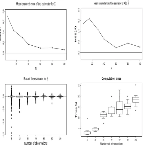
We consider the different sample sizesN = 5,15,30,40,60,80,100 and we simulateM = 100 replicates for each value of the sample size. We estimate the mean squared error asMSE[_N(Σ) =b _M¹ ∑_M

i=1d_R(Σb_N,i,Σ)²andMSE(A((1,[ 1);,β)) =b

1 M

∑M

i=1||log_Σ(exp_Σb

N,i(A((1,1);βb_N,i))) −A((1,1);β)||²F, where Σb_N,i and βb_N,i are the estimates for thei-th replicate with sample size N. The estimated mean squared errors can be seen in Fig. 1 , alongside the computation times. The MSEs approach zero when the sample size increases, thus suggesting empirically that the proposed estimator are consistent. We report in Fig. 1 also the boxplots of the biasβb_N,i−βfor the regression coefficients. Their estimates appear to be unbiased for largeN. This is not surprising, since the estimators forβ would be unbiased ifΣwas known and we have seen thatΣb_N becomes closer and closer to Σwhen N increases. However, for finite sample sizes we expect the need to estimateΣ to add some bias on the estimators for the regression coefficients. Finally, we can see that the computation times (obtained running an R code on an Intel i5-4690K CPU 3.5GHz machine) for the estimator increase with the sample size but only linearly.

We want now to assess the performance of the proposed method for kriging prediction, which is the our final goal. We independently simulateM = 100real- izations from a2×2positive definite matrix random field defined on the bidimen- sional spatial domainDand consistent with model (7), where errors are spatially correlated. The two diagonal elements and one of the off-diagonal elements of the error matrix in the tangent space are independent realizations of a real valued, zero-mean Gaussian field with Gaussian variogram of decay0.1, sill0.25and zero nugget. The remaining off-diagonal element is determined by symmetry.

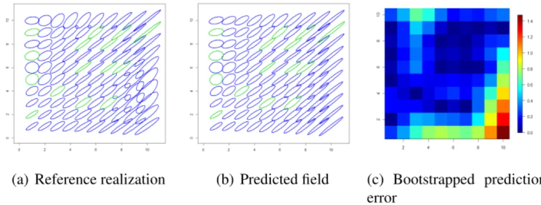
We generate the realizations of the random field on a10×10regular grid of locations and we observe the field in15randomly selected grid pointss₁, ...,s₁₅; these15locations are kept fixed across theM simulations.

Fig. 2 shows the results obtained for the first simulation: the reference real- ization is shown in panel (a), the predicted field in panel (b) and the expected prediction error assessed through (12) in panel (c). In Fig. 2a and 2b, each2×2 positive definite matrixSobserved or predicted at a locationsis represented as an ellipse that is centered in sand has axis√σ_je_j, whereSe_j =σ_je_j, forj = 1,2.

Overall, the pattern of the reference realization appears to be fairly captured by the kriged field. Only the bottom right corner of the spatial domain seems to be affected by a significant prediction error, due to the absence of data near this

20 40 60 80 100

0.00.20.40.60.8

Mean squared error of the estimator for Σ

N

MSE(Σ^)

20 40 60 80 100

0.00.20.40.60.8

Mean squared error of the estimator for A(1, β^)

N

MSE(A^)

5 15 30 40 60 80 100

−1.5−1.0−0.50.0

Bias of the estimator for β

Number of observations

5 15 30 40 60 80 100

510152025

Computation times

Number of observations

Times (s)

Figure 1: MSEs of the estimatorsΣb(top left) andA((1,1);,βb)(top right) and element-wise bias on the regression parametersβb−β(bottom left) as a function of the sample size and corresponding computation times (bottom right), obtained running an R code on an Intel i5-4690K CPU (3.5GHz) machine.

(a) Reference realization (b) Predicted field (c) Bootstrapped prediction error

Figure 2: Panels (a) and (b): Comparison between the reference realization of the matrix field and the predicted field. Each positive definite matrix is represented by an ellipse centered in the respective location. Observed data are represented in green. Panel (c): Estimated expected prediction error.

boundary of the domain. This is reflected by the estimated prediction error (Fig.

2c).

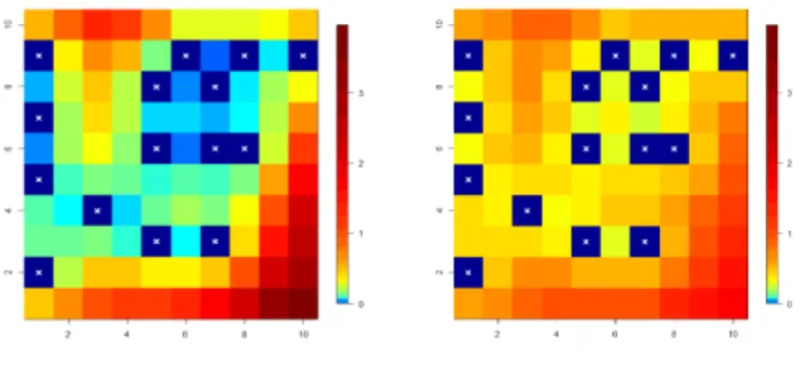
To evaluate the goodness of the estimator (12) for the expected prediction er- ror, we use the M = 100 independently simulated field realizations as follows.

For every simulation, in each of the 85 grid locations different froms₁, ...,s₁₅,we compute both the kriging prediction secured by the estimator (11) and the esti- mate of the expected prediction error achieved by (12), having setB = 100to be the number of bootstrap replicates. Fig. 3 compares the maps of: (a) the average prediction error across the M = 100 simulations, i.e. the average of the square distance between the known field realization and its kriging prediction, and (b) the average, across the sameM = 100 simulations, of the estimates of the expected prediction error supplied by the estimator (12). It can be noticed that the semi- parametric bootstrap estimator provides a good evaluation of the prediction error, with only a slight overestimation near the observed locations.

In the remaining part of the section, we illustrate a second simulation study aiming at evaluating the performance of the kriging predictor when data are gen- erated from a model different from (7). In particular, we follow Pigoli and Secchi (2012) to generate a non stationary matrix field according to a probabilistic model with meanP(s) = exp_Σ(A(x(s);β)), whereΣandA(x,β)are set to be the same as in the previous simulation study. This random matrix field is obtained through

(a) Average prediction error across100simulations

(b) Average estimate of the ex- pected prediction error across the same 100 simulations

Figure 3: Comparison between the average prediction error, computed across100simulations, and the average estimate of the expected prediction error. Crosses indicate the position of the observed locations.

the sample covariance matrices generated by the realizations of a Gaussian ran- dom vector fieldv.

LetD⊂R²indicate the common spatial domain of two independent gaussian random fieldsw(s),y(s), s∈D.Both random fieldswandyhave zero mean and Gaussian spatial covariance with decayϕ = 0.1, sill equal to 1 and zero nugget, i.e.

Cov(w(s_i), w(s_j)) = Cov(y(s_i), y(s_j)) =

{ exp(−ϕ∥s_i−s_j∥²) ∥s_i−s_j∥² >0, 1 ∥si−sj∥² = 0,

(13) for s_i,s_j ∈ D. For s ∈ D, the covariance matrix (between components) of the random vector field v(s) = (P(s))¹²(w(s), y(s))^T is equal toP(s). We generate N independent realizations of the random vector field v and, for s ∈ D, we compute the sample covariance matrix

S(s) = 1 N −1

∑N k=1

(v_k(s)−v(s))(v¯ _k(s)−v(s))¯ ^T ∼Wishart₂ ( 1

N−1P(s), N −1 )

, (14)

¯

v(s)being the sample mean ins∈D.

For N = 4,5,6, we replicate the simulation M = 25 times on the same 10×10 regular grid of the first simulation study described in this section. For

each simulation, we observe the realizations of the field S in the same 15loca- tionss₁, ...,s₁₅ selected in the first simulation study and we then predict the field realizations in the remaining 85 locations through the kriging estimator (11). Note that the parameter N controls the marginal variability of the matrix random field S.

We evaluate the performance of the kriging procedure when applied to these simulated fields by comparison with the case when data are generated by model (7). Thus, we generate a second set of M = 25simulations using model (7) and setting the value ofVar(∆) = σ² = 0.35,1,1.9.This provides field marginal vari- abilities comparable to those of the random fields generated by model (14) when N = 6,5,4,respectively. Indeed, it is fair to compare prediction performances when the marginal variabilities of the random fields which generate the data are close. However, it is not trivial to obtain an explicit relationship between the pa- rameters controlling the field marginal variability in the two models, i.e., N and σ².

Thus, for both models we measure the empirical mean square error with re- spect to the mean of model (14), expressed by ς = ₁₀₀¹ ∑100

i=1d(S(s_i), P(s_i))², and the average prediction error expressed byp¯= ₈₅¹ ∑85

i=1d(S(s_i),S(sb _i))². Each point in Fig. 4a represents the joint values of ς andp¯relative to one of the 150 simulations considered in this study: red points are relative to the 75 simulations - 25 simulations for each of the three values chosen for the parameter N - when data are generated by model (14), while black points are relative to the 75 simu- lations - 25 simulations for each of the three values chosen for the parameterσ² - when data are generated by model (7). Polynomial smoothing lines are added to help visual comparison. Inspection of Fig. 4a suggests that the performance of the kriging predictor (11) when model (7) is violated is worse than its performance when model (7) is correct. Moreover, the higher the value ofς the worse is the rel- ative performance of the kriging predictor. This is to be expected because a high dispersion on the manifold means that no tangent space can accurately describe the data. However, for low values ofς the performance of the kriging predictor in the two situations is comparable, supporting its robustness to the violation of the model provided that the tangent space approximation is able to describe in a fairly accurate way the observations.

By way of example, Fig. 4b and 4c represent two realizations of the matrix field generated from (14) for high and low values of N, respectively, i.e. low or high values of the field empirical marginal variabilityς.

In all the above simulations we use a Gaussian covariance function, since this

(a) Prediction error and variability

(b) Field realization withς = 2.9 (c) Field realization withς = 6.7

Figure 4: Panel (a): Prediction error as a function ofς, with a local polynomial smoothing added to help visual comparison, for data generated from the tangent space model (7) (black points and solid black line) and from procedure (14) (red points and dashed red line), both with Gaussian covariance function. Panel (b) and (c): Examples of simulated fields from model (14) forN = 6 (b) andN = 4(c) and Gaussian covariance function, with the respective values ofς.

appears to be the most suitable model for spatial dependence in the case study we analyze in Section 5. However, the Gaussian model has a particularly smooth be- haviour that can be sometimes misleading as a test case, see Stein (1999, Section 2.7). For this reason, we also replicate the same simulations using an exponential covariance function, both in the tangent space model and in equation (13). The results can be found in the Supplementary material and they are very close to the ones obtained in the Gaussian case.

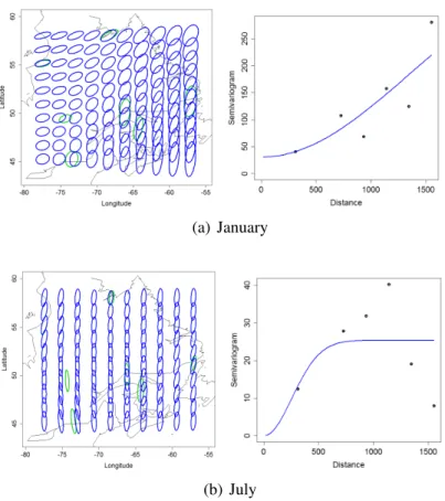
5. Kriging for Quebec meteorological data

In this section a kriging interpolation is proposed for the covariance matrices between temperature and precipitation in Quebec. The co-variability of temper- ature and precipitation is of great interest for meteorological purposes, since a good understanding of their relationship can improve weather forecasting meth- ods. Moreover, relative behavior of temperature and precipitation affects agricul- tural production (see Lobell and Burke, 2008). For a detailed description of the temperature - precipitation relationship and its estimate see, e.g., Trenberth and Shea (2005) and references therein.

We focus on the Quebec province, Canada. Data from Canadian meteorolog- ical stations are made available by Environment Canada on the website http:

//climate.weatheroffice.gc.ca. We restrict to the 7 meteorological stations where all monthly temperature and precipitation data are available from 1983 to 1992. For each station and for each month from January to December, we use these10-year measures to estimate the2×2 covariance matrix between temperature and precipitation. We thus obtain and separately analyse 12 datasets, each composed by n = 7spatially dependent sample covariance matrices (with the previous notation, n = 7 and p = 2). These datasets have been previously considered in Pigoli and Secchi (2012) with the aim to estimate a regional covari- ance matrix starting from the observations coming from different meteorological stations. Here, the aim of the analysis is different, since we want to predict the co- variance matrix in unobserved locations, starting from the incomplete realization of the field.

For the analysis, we choose the affine invariant Riemannian metric as the dis- tance between covariance matrices because of its invariance property to changes in the measurement units. At first, we make the hypothesis of stationarity for the random field (i.e., that the matrix random field has a constant mean), thus includ- ing only a constant term in the tangent space model. A Gaussian semivariogram model with nugget seems appropriate to fit the empirical semivariogram in the