The standard finite element method in the frequency domain is found to be unsuitable for the analysis of multimode applicators containing food-like materials due to the severe ill-conditioning of the matrix equations. A brief overview of the methods available for solving linear equations is given.
Microwave Energy: Volumetric and Selective Heating
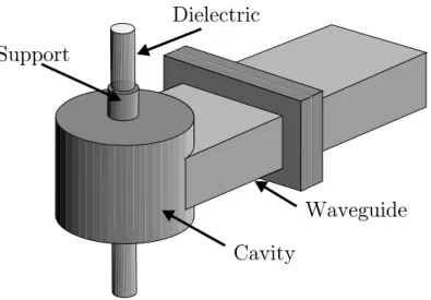
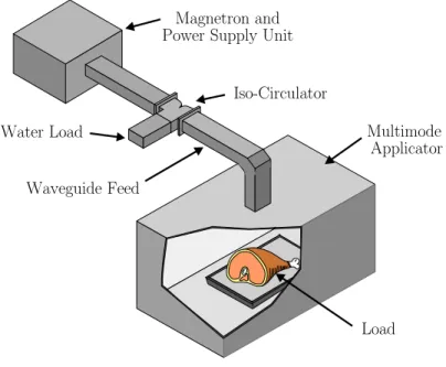
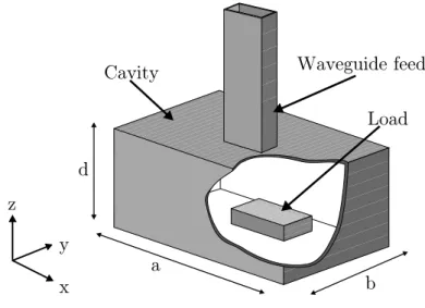
An iso-circulator [Metaxas & Meredith, 1983] is used in the feed to absorb any reflections from the cavity. Simulation can assist in the design of these applicators by predetermining the heating pattern.
Microwave Applicators
Single Mode Resonant Cavities
The dimensions of the cavity are chosen so that the resonant frequency of this mode coincides with the frequency of the source when the applicator is loaded. It is possible that the loading causes certain higher order modes to be excited, in which case the field pattern will differ from that of the dominant mode.
Multimode Cavities
This means that it is necessary to calculate the response of the system at a range of different frequencies. Uneven heating can therefore cause a thermal runaway that leads to the destruction of the sample being heated [Metaxas & Meredith, 1983].
Applicator Design
A further complication arises because the behavior of the source is generally dependent on the load to which it is connected. The frequency of operation is also dependent on the impedance of the load to which it is supplying power.
Computational tools
Analytical Methods
If the plate extends over the entire cross-section of the cavity, i.e. the inhomogeneity is only in one dimension, then analytical expressions for the resonant modes can be found [Paoloni, 1989]. It is then assumed that the source field distribution can be expanded as a Fourier-like sum of modes.
Numerical Methods
The finite element method is one of the most versatile methods available to the numerical analyst. Its ability to use irregular conformal meshes was one of the main reasons for choosing the finite element method in this work.
Experimentation and Verification
Another approach that is often taken and will be used later in this thesis is to measure the temperature rise in the load being heated. The thermal camera can only record surface temperatures and taking measurements while the load is being heated is difficult.
Computer Implementation
Governing Equations
Eliminating H from (2.7) and (2.8) gives the vector Helmholtz equation;. 2.9), which is used to discretize the frequency domain.
Spurious modes
Finite Element Discretisation
Traditional Nodal Elements
1987] suggest that two variables can be used for the normal component of the field at dielectric interfaces. 1994a] is to use edge elements near sharp metal corners and node elements in the body of the domain.
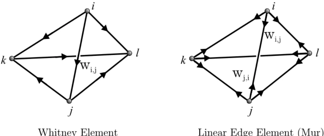
Edge Elements
This approach is claimed to offer the flexibility of edge elements along with the accuracy and economy of nodal elements. It may therefore be desirable to use hexahedral edge elements so that the hexahedral mesh can be used unmodified.
Frequency Domain Finite Element Method
Time Domain Finite Element Method
- Introduction
- Formulation
- Stability
- Lumping
For the system to be stable, the roots of (2.35) must then lie in the left half of the z-plane. Therefore, for the clumping to work satisfactorily, it is necessary to ensure that the elements of the mesh are of high quality.
Boundary Conditions
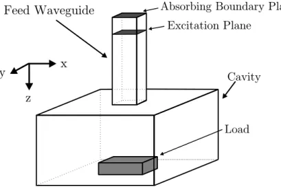
Absorbing boundary conditions (ABCs)
The ABC used here simply involves terminating the waveguide at its characteristic impedance, which can be done by evaluating the surface integral term of equation (2.22) [Dibben &. The connectivity remains unchanged, so that the sparsity of the matrix is not reduced and the matrix remains symmetric.
Post-Processing of Edge Element Results
Error calculation
To assess the error from a given discretization, it is necessary to define a measure of this error. The one used here is the `2-norm, which for a vector space y is defined by,.
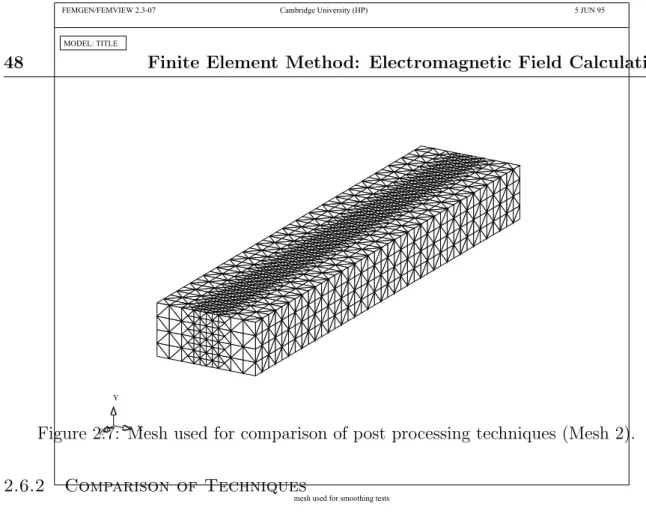
Comparison of Techniques
Comparison of Element Types
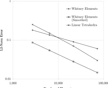
Comparison of Whitney Elements and Linear Edge Elements
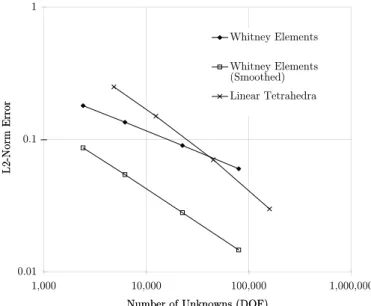
To determine the relative errors of the two elements, an empty waveguide (WG9A) was modeled. However, when the post-processing is performed, the convergence rate of the two elements becomes very similar and Whitney elements give a consistently lower error than the linear elements.
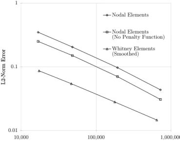
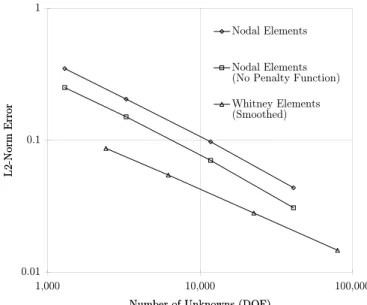
Comparison of Whitney Elements and Nodal Elements
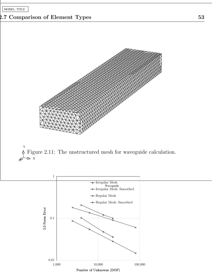
From Figure 2.9 it is clear that for a given error Whitney elements produce a significantly smaller coefficient matrix than linear elements providing much greater efficiency. The error produced by the irregular mesh is slightly larger than that of the regular mesh, shown in Figure 2.12, however, the convergence properties remain the same.
Comparison of Edge Element Shapes
Conclusions
The purpose of this chapter is to describe some of the methods that can be used to solve (3.1) and compare their performance. Methods that are suitable for the finite element problem are first discussed, then various preconditioning techniques that can be used to speed up the convergence of the iterative techniques are outlined.
Direct Methods
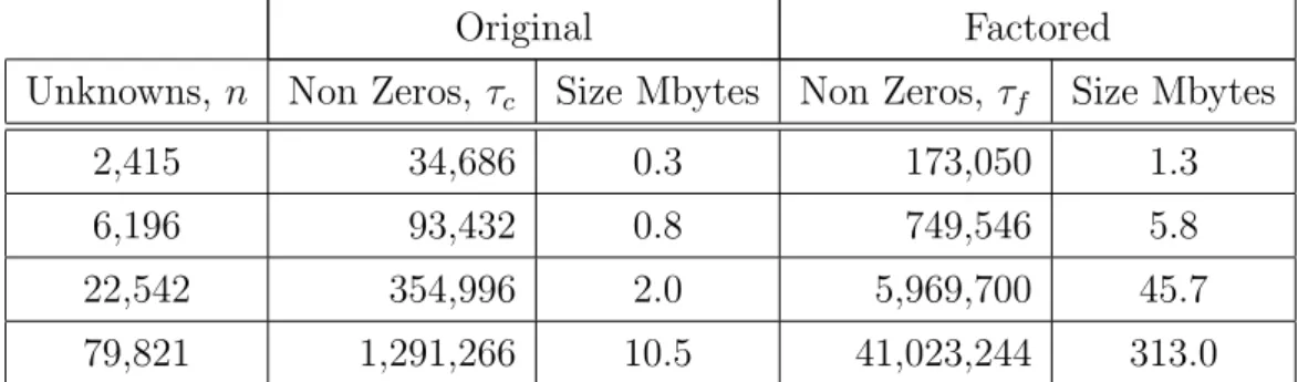
One of the most effective methods for finite element calculations is the minimum degree algorithm. The size of the coefficient matrix increases as O(n) while the factored matrix increases as ~ O(n1.6) in this case.
Iterative Techniques
- Introduction
- Complex Systems
- Preconditioning
- Terminating Criteria
This method no longer satisfies the minimization property of the conjugate gradient algorithm [Barretet al., 1993]. If the original matrix is splitA=D−B, where D is the diagonal of the matrix, the factorization is applied to the system.

Ill-Conditioning
Estimation of the Condition Number
An accurate calculation would require forming the inverse, a process that is very computationally expensive. Many alternative methods of estimating the conditional number have been proposed that avoid the generation of the inverse.
Application to the Frequency Domain Method
Single Mode and Waveguide Problems
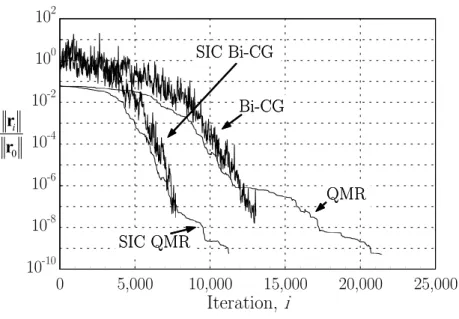
The condition number is dependent on both the mesh discretization and the nature of the problem being modeled. In general, the number of iterations for the solution gives a better indication of the efficiency of the method since it will be machine independent.
Multimode Cavity Problems
The main difference between meshes 2 and 3 is the discretization of the air in the cavity. As the load permittivity increases, the convergence of the SIC-QMR method gradually becomes slower.
Application to the Time Domain Method
- Diagonal Scaling
- Direct Methods
- SOR Iteration
- Preconditioned Conjugate Gradients
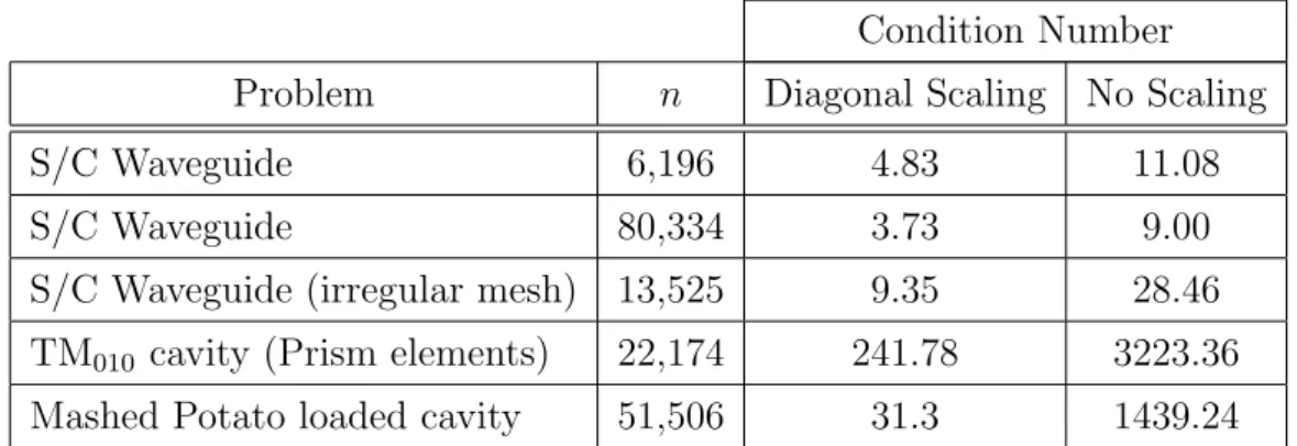
If node elements were used, the condition number of the mass matrix ( [T²]) becomes independent of both the element size and shape and the size of the mesh [Wathen, 1987]. Scaling has the effect of removing the dependency of the condition number on material properties.
Conclusions
Some of the energy supplied to the applicator will be reflected back to the source. The calculation of the amount of reflected energy is necessary to determine the amount of energy that will be absorbed by the load being heated.
Calculation of Reflection Coefficient
The qab2 term appears in equations (4.1) and (4.2), so that the integral over the waveguide cross-section, S, of the eigenvector of the TE10 mode is normalized [de Pourcq, 1984]. The integrals (4.11) and (4.12) are then calculated from the summation of the integrals over each surface on two different planes respectively.
Power Calculation
Power Calculation by E-Field Scaling
The power flowing in the waveguide is given by the integral of the Poynting vector over the cross-section of the waveguide. Replacing the E and H fields with the TE10 mode using equations (4.1) and (4.2) and considering only the forward wave gives. 4.19) where A0 is the magnitude of the forward wave at power Pf.
Power Calculation by Scaling Total Power
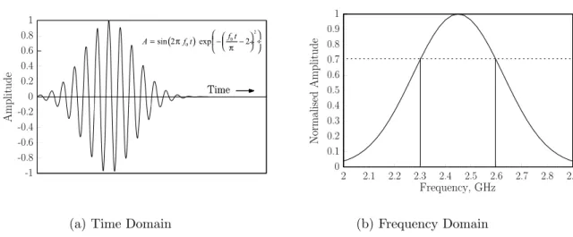
Gaussian Pulse Excitation
In practice, however, storing all the field values at each time step would require a huge amount of disk space, so the DFTs at selected frequencies accumulate during the time step process. This determines the rate of decay of the stored energy, W, in the system after any excitation is removed.
Signal Processing Techniques
It remains to be seen whether these techniques can be successfully applied to the microwave heating problem. This allows the results obtained here to be compared with the solutions of other workers using different methods.
Rectangular Cavities
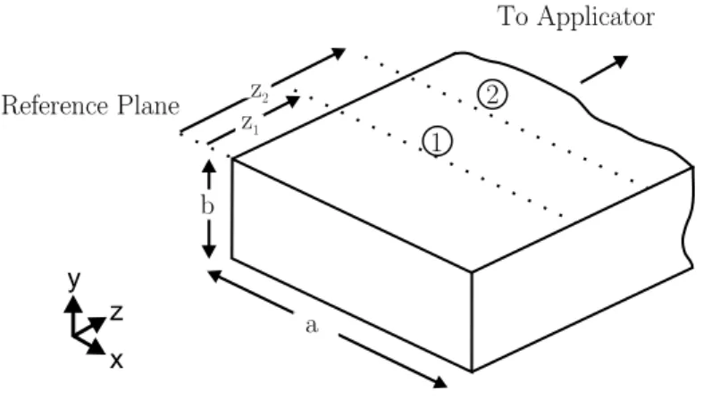
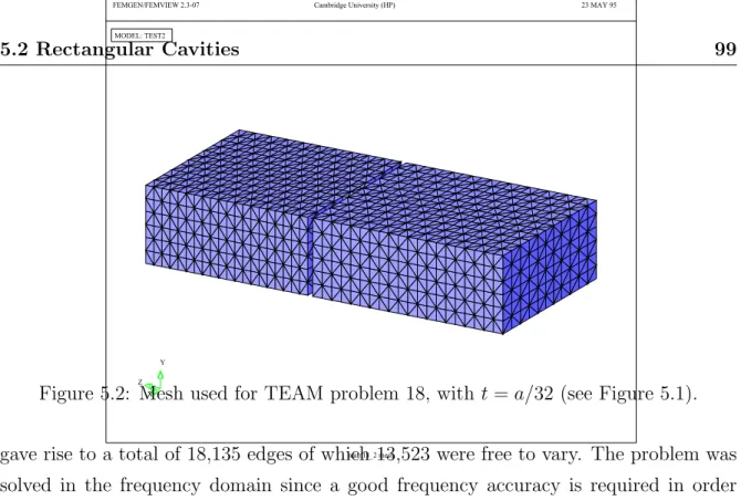
Waveguide Loaded Cavity: TEAM Problem 18
The calculated phase of the reflection coefficient on the input plane is shown in Figure 5.3(a). The magnitude of the reflection coefficient is the same at all frequencies, since the system is lossless.
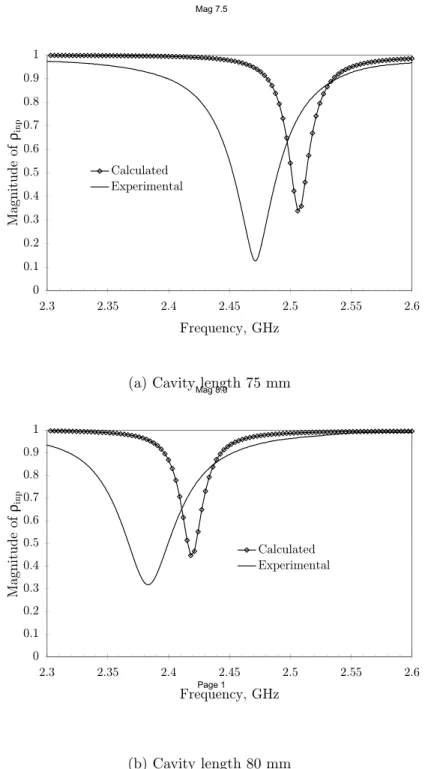
Experimental TE 101 Applicator
It is clear from Figure 5.6 that as the time step is reduced, the accuracy of the solution increases, which is to be expected. The finite element method will always yield a unit magnitude for the reflection coefficient of the empty cavity when the walls are assumed to be perfect conductors.
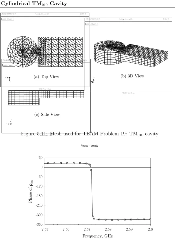
Cylindrical TM 010 Cavity
TM 010 Cavity: TEAM Problem 19
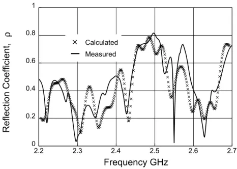
The phase angle and magnitude of the reflection coefficient at the entrance face for the empty cavity are shown in Figure 5.12 for an iris width of 15 mm. The magnitude and phase of the reflection coefficient at the entrance plane are shown in Figure 5.13 and the electric field distribution at resonance in Figure 5.14.
Experimental TM 010 Cavity
The network analyzer was calibrated using a waveguide calibration set so that the reference plane was located on the flange of the coaxial to waveguide transition. For the calculation, it was assumed that water has a relative permittivity of 77−12, which is that of pure water [Metaxas & Meredith, 1983], whereas ordinary tap water was used for the experiment.

Conclusions
The results show that by decreasing the time step size, the results of the time domain method approach the results of the frequency domain with a difference of only 0.03% when using 60 steps per cycle. It appears that the results are very sensitive to small changes in frequency and to changes in the dielectric properties of the material.
Mesh Generation
Adaptive meshing
It is also possible for the field solution to drive mesh generation: a process known as adaptive mesh refinement. The network is then refined in those areas where the error is considered to be too high and the process is repeated.
Experimental Setup
Thermal Imaging Technique
The process of transferring the charge from the cavity to a suitable position for thermal imaging was quick, requiring only a few seconds. Since the images were stored electronically, it was possible to use the same graphics package to display the thermal images and the calculated results.
Mashed Potato Loaded Cavity
The electric field distribution on a vertical slice through the center of the cavity is shown in Figure 6.7. The power density at the top of the potato and for a vertical cut through the middle of the tray is.
Pastry Block
In the upper part of the block, the heating is concentrated in the four corners, which is correctly predicted by the model. The value obtained in this way is compared with the numerically calculated value in figure 6.10.
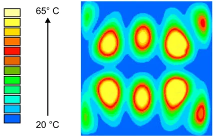
Plastic Block
- Introduction
- Experimental Results
- Solution at a Single Frequency
- Multiple Frequency Solution
- Effect of Lumping
- Solution with a Fine Mesh
- Effect of Variation in Dielectric Properties
- Discussion of Results
The peaks in the center of the cavity are slightly higher for the frequency domain calculation, but otherwise the solutions are identical. The thermal image in Figure 6.11 has six hot spots in the central region of the block as calculated.
Conclusions
Second, changes in both the real and imaginary parts of the permittivity will affect the electric field distribution. In these cases, the electric field distribution within the applicator will almost certainly vary with the temperature of the load.
Solution of the Heat Flow Equation
7.7) where λi are the shape functions within the element and qvk is the value of the power density at the node. Inside the material, the contributions to [H] and [R] from adjacent elements will cancel, so they are non-zero only for the faces of the elements that are on the surface of the material.
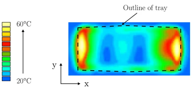
Temperature Distribution in Mashed Potato Load
This is especially noticeable along the edges at the end of the tray, as the heat loss at these points will be from two sides. The model was not able to take into account the tray in which the potato was contained.

Coupled Electromagnetic and Thermal Models
Introduction
The results in Chapters 5 and 6 for the reflection coefficient show large changes in magnitude with frequency. This will also give an indication of the sensitivity to errors in the reflection coefficient.
Temperature Feedback
This suggests that the system should also be solved at different power levels to determine the sensitivity to changes in absorbed power. If the system is operating close to a sharp resonance, a small change can cause very large changes in the reflection coefficient and thus in the absorbed power.

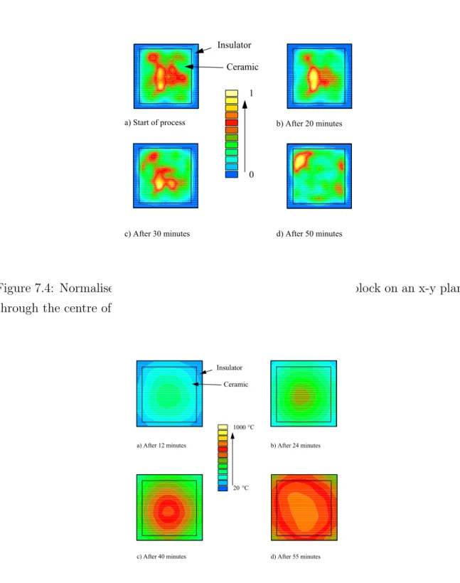
Ceramic Block Example
Conversely, if too large a change is allowed before recalculation, the evolution of the temperature distribution will be altered. If the system is operating close to a sharp resonance, a small change can produce very large changes in the reflection coefficient and therefore in the absorbed power. a) Start of process b) After 20 minutes.
Conclusions
The most important part of this thesis is the development of the time domain finite element method for solving multimode cavity problems. An iteration method for solving the eigenvalue problem of linear differential and integral operators.