Design synthesis of NLMPC-based tracking controller for autonomous vehicles with active aerodynamic control

Furthermore, I hereby declare that I am the sole source of the creative works described in this dissertation. 60 Table 4.3: Performance measures of the nominal and optimal designs for both the urban and highway cases.

Introduction

Background and Motivation

These additional downward forces will be counted towards the vertical load on the tires and therefore improve the maximum adhesion of the vehicle [9]. The active aerodynamic control system is composed of four independent NACA-0012 spoilers, and one spoiler is installed above each wheel located at four corners of the vehicle.

Thesis Objectives

The design variables for the mechanical vehicle can be inertial and geometric parameters, while the design variables for the tracking controller can be weighting factors. In both vehicle models, the nonlinear magic formula tire model is used to simulate the tire-road interactions, and these vehicle models are applied as a prediction model for the design of the NLMPC-based tracking controller.

Thesis organization

Literature review

Autonomous driving systems

Vehicle aerodynamics

Vehicle system dynamics

Model predictive control

Particle swarm optimization

Research gaps identified from the literature review

Design synthesis method

Proposed design synthesis method

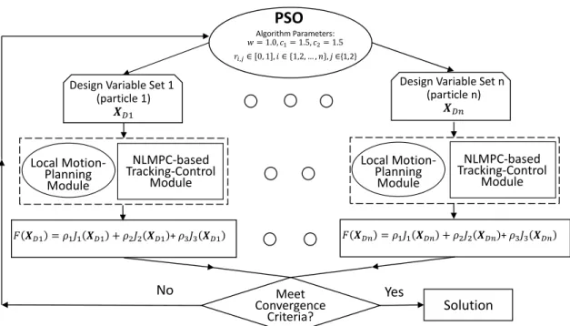
On the top layer there is an optimization that uses the PSO or GA algorithm, while on the bottom layer there are the associated components of the motion planner, NLMPC controller and virtual vehicle. This section introduces the structure and functionality of the proposed design synthesis method, which includes the PSO algorithm, vehicle models, and NLMPC controller design.

Structure of proposed design synthesis method

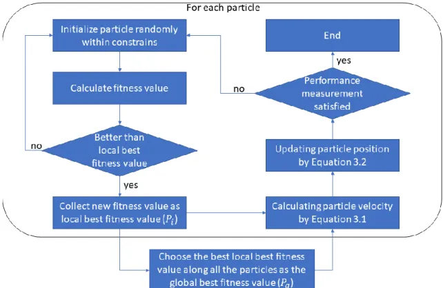
As introduced in literature review, the MBK-based tracking control is itself an optimization problem. The use of a two-layer optimization technique for the design of mechatronic vehicles usually leads to a complex non-convex optimization problem, where a variation of the initial conditions can result in different design solutions [92]. In this research, a PSO algorithm is used for solving the upper layer optimization problem shown in Figure 3.1.

Optimizer at upper layer – PSO

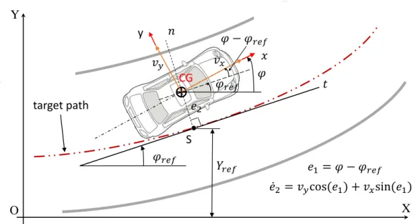
As shown in Figure 3.4, it is possible to determine the position and orientation of the vehicle relative to the target path at a given moment. In this study, the parameter values ​​of the 3-D CarSim model are listed in the Appendix. As shown in Figure 3.6, an independent NACA-0012 spoiler is installed at each corner of the vehicle.

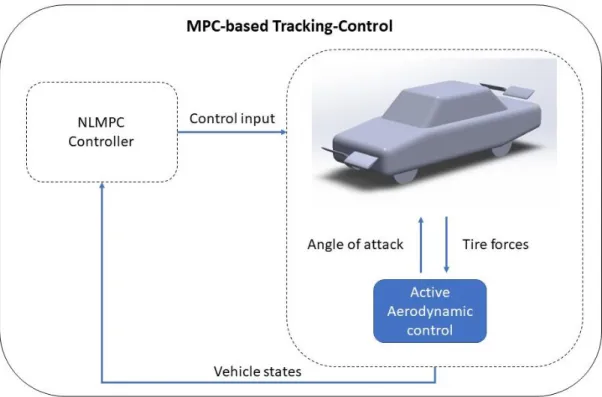
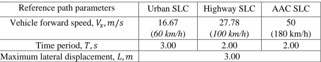
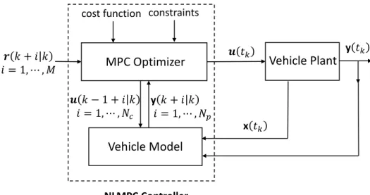
To summarize the design of the NLMPC controller, the interrelationships between the controller and the vehicle plant are visualized using the block diagram in Figure 3.13. For the application of high-speed vehicles, the implementation of the proposed design synthesis method is similar to that shown in Figure 3.14. For the three case studies, the values ​​of the reference path parameters are shown in Table 4.1.

The virtual vehicle plant with the AAC system, and the resulting vehicle plant is used for the design of the NLMPC tracking controller.

Vehicle models

• CarSim model without active aerodynamic control
• CarSim model with active aerodynamic control
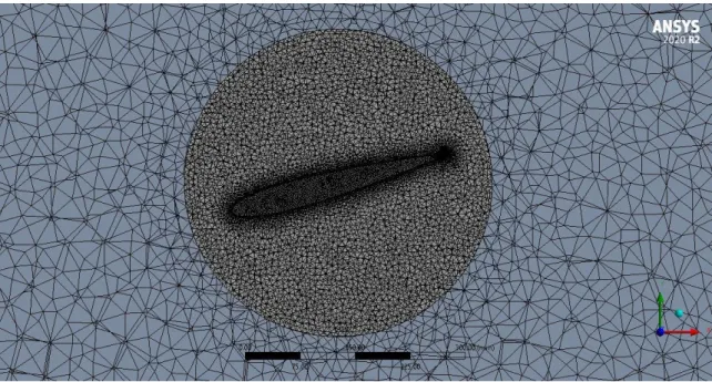
• Spoiler modelling
• Meshing
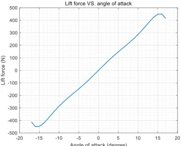
• CFD results

Nonlinear model predictive control

The NLMPC controller consists of two core elements: the discretized vehicle model represented by Equations (3.13) to (3.15) and an optimizer with a cost function and a set of constraints. With the prediction, optimization is performed to find a sequence of control input movements that minimizes the chosen measures of the output deviation from their respective reference trajectories while satisfying all the given constraints. To improve the quality of the prediction, appropriate measurements are collected; however, only the first of the calculated control input sequences is implemented.

To design the NLMPC controller, we need to discretize the nonlinear vehicle model described in Equation (3.11). Following the directives of the behavior planner, the local motion planner generates the reference trajectory (i.e., r(∙)) for the NLMPC controller to manipulate the tracking action, as shown in Figure 3.13. In contrast, the disjoint methods significantly improve the computational efficiency due to the layered nature [98].

To facilitate systematic and repeatable testing of the proposed design synthesis method, it is assumed that the local motion planning results in an SLC path at a given speed.

Implementation of The Design Synthesis Problem

• Design objectives, variables and constrains
• Implementation of the bi-layer optimization problem
• Implementation for high-speed vehicles with active aerodynamic control 56

2 (3.20) where 𝐽1 represents the root mean square (RMS) value of the vehicle lateral path deviation, 𝑒2, over the SLC maneuver. Reliable guidelines for choosing the tuning parameters of the forecast horizon, 𝐻𝑝, and control horizon, 𝐻𝑐, are well established [82]. With the above considerations, we treat the elements of the weight matrices 𝑸 and 𝑹 as the components of the design variable subset 𝑿𝐷𝑚.

To facilitate the design optimization, each term of the right-hand side of Equation (3.27a) is normalized with the respective norm [76], [77]. For the case in question, the norm of each term is the inverse of the respective weighting factor, that is. About the SLC maneuver, the NLMPC controller determines the steering angle 𝛿 of the vehicle plant (defined by Equation (3.11)) to track the reference path at a constant forward speed.

By performing the equivalent SLC maneuver corresponding to each of the n sets of design variables, the vector of fitness values, [𝐹(𝑿𝐷1), 𝐹(𝑿𝐷2),.

Case studies specification and testing maneuvers

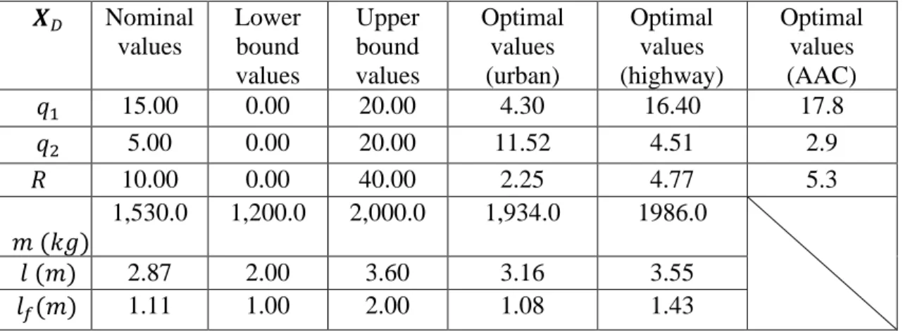
Therefore, the number of design variables in the case of AAC is three (i.e., controller parameters only), while the other two cases have six design variables (i.e., controller parameters and vehicle parameters). Note that the design optimization is implemented independently in the three cases, i.e., city, highway and AAC. To implement these design optimizations, both the population number (i.e. the total number of particles), n, and the total number of generations of the PSO algorithm are assigned the value 100.

After performing design optimizations according to three operating scenarios, optimal sets of design variables and corresponding performance measures defined in equations (3.20) to (3.22) are achieved. To analyze and evaluate the achieved optimization results, co-simulations are carried out with the integration of a virtual vehicle, i.e. of the CarSim model, with associated motion planning modules and NLMPC tracking-control modules designed in Matlab. In the following subsections, the co-simulation results are first examined in terms of nominal and optimal design performance measures in all three cases, and then the effects of optimal design variables on performance improvements are evaluated.

Performance measures of urban and highway scenarios

It is clear that the fluctuation of the lateral acceleration in the nominal design is more violent with larger peak values ​​than its counterpart in the optimal design. As expected, each of the control inputs takes a single cycle sine wave form for the SLC maneuvers. A close observation of Figure 4.9 shows that the total steering control effort for the optimal design is greater than its counterpart for the nominal design.

All the aforementioned performance measures for the nominal and optimal designs as well as their relative variations are listed in Table 4.3. The performance improvement of the optimal design can be attributed to its greater steering effort on the front wheel. In the case of the highway scenario, the respective performance measures for the nominal and optimal designs are also given in Table 4.3.

Interestingly, the performance improvement of the optimal design compared to the nominal design in the highway scenario is similar to that in the urban scenario.

Performance measures of high-speed case with AAC

From Figures 4.11 to 4.15, the performance improvement of the optimal AAC design compared to the nominal design has similar implications as those for the urban and highway scenarios. All performance measures of the nominal, optimal, and optimal AAC designs and their relative variations are listed in Table 4.4. In order to identify the effects of spoilers, the three models are again compared in these images.

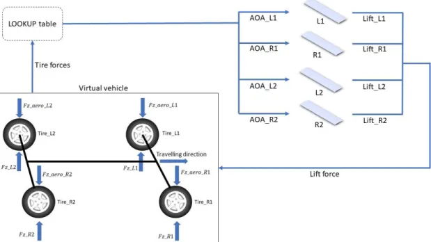
Figures 4.16 and 4.17 show the vertical variation of tire force (tire L1 and R1) on the front axle, while Figures 4.18 and 4.19 show the vertical variation of tire force (tire L2 and R2) on the rear axle. Table 4.4 listed three important performance measures of the AAC system: the maximum vertical force difference in the front axle tires (𝐹𝑧_𝑑𝑖𝑓𝑓_𝑓𝑟𝑜𝑛𝑡_𝑚𝑎𝑥), the maximum. These three measures can accurately describe the difference in vehicle roll dynamics due to the effects of the nominal, optimal, and optimal with AAC designs.

It is clear that the performance of the optimal design with AAC outperforms that of nominal and optimal designs without AAC.

Effects of design variables

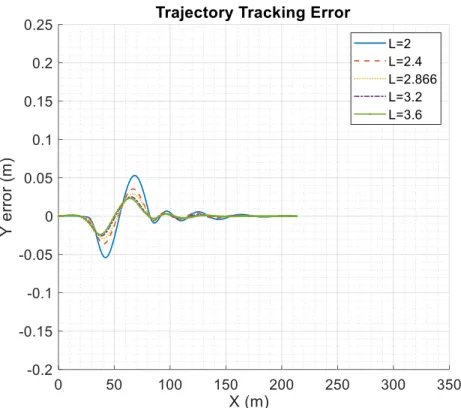
A close observation of figure 4.23 reveals that the larger the 𝑙 value becomes, the smaller the maximum peak 𝑌𝑎𝑤_𝑎𝑛𝑔𝑒𝑟𝑟 value will reach. However, in the USLC case as shown in Figure 4.22, the above conclusion derived from the observation based on the result illustrated in Figure 4.23 is not true. It is shown that with the variation of 𝑞1, the change of the two peak values ​​of 𝑌𝑒𝑟𝑟 is not obvious.

In the case of HSLC (as shown in Figure 4.25), it is observed that the larger the weight of 𝑞1, the larger the maximum peak 𝑌𝑒𝑟𝑟. By imposing a penalty on the size of 𝑌𝑎𝑤_𝑎𝑛𝑔𝑒𝑟𝑟, increasing the weight value of 𝑞1 leads to a decrease in the maximum peak. In addition to the above sensitivity and vehicle dynamics analysis, the effects of the other individual design variables, including 𝑞2, 𝑅, 𝑚, and 𝑙𝑓, on the performance measures of 𝑌𝑒𝑟𝑟, 𝑌𝑎𝑤_𝑎𝑛𝑔𝑒𝑟𝑟, and the RMS value of 𝑎𝑦, respectively .

Comprehensive vehicle sensitivity and dynamics analysis justifies optimal road vehicle designs with autonomous driving functions in both USLC and HSLC scenarios.

Conclusions

Conclusions

A special case is performed under high-speed operating conditions considering the application of the active aerodynamic control function. The lift/down forces of the vehicle's aerodynamics and the corresponding dynamic effects at high speeds, e.g., 180 km/h, are simulated in a high-speed SLC maneuver. This case study aims to test the active aerodynamic control design with the installation of four independent spoilers.

The virtual vehicle system utilizes the aerodynamic properties of the spoilers to improve the vehicle's stability and handling. The simulation results indicate that the AAC system can improve high-speed handling and driving characteristics in terms of path-following off-tracking, cornering stability, ride quality, vertical tire force transformation and roll stability.

Future research work

Longitudinal, lateral and lateral movements are essential in the design and analysis of treatment characteristics. An active vehicle control system uses the subsequent results from the study of the vehicle's dynamic characteristics.