Essays on experimental economics: preference Reserval and networks

Texto completo

(1)ESSAYS ON EXPERIMENTAL ECONOMICS. PREFERENCE REVERSAL AND NETWORKS. BASAK GUNES. TESI DOCTORAL UPF / 2009. DIRECTOR DE LA TESI. Prof. Rosemarie Nagel (Universitat Pompeu Fabra).

(2) To my mother Without her, this would not have been possible.... iii.

(3)

(4) Acknowledgements Studying in Barcelona for a PhD degree will always constitute a big chapter in my life. This thesis is a product of these past five years spent on this challenging path. Then again, it would be impossible to handle it all if it was not for those people that I am indebted to. This dissertation could not have been written without Rosemarie Nagel who not only served as my supervisor but also encouraged and challenged me throughout my academic program. She and many other academic researchers have guided me through this process. I am grateful to Antonio Cabrales whose opinion and advice have always been indispensable. My thesis has also advanced and come to this point through the invaluable insights I have acquired in my talks with Yann Bramoullé, Joan De Martí, Fabrizio Germano, Robin Hogarth, Nagore Iriberri and Marc Le Menestrel. I thank them all. I also would like to extend my heartfelt gratitude to Shikeb Farooqui, Aniol Llorente-Saguer, Yusufcan Masatlioglu and Neslihan Uler for all the suggestions they gave me on improving this thesis. I am also thankful to Joerg Franke and Tahir Ozturk for their contributions to the second chapter. I am especially indebted to Zeynep Gurguc for her diligent work in the second chapter and her unremitting support throughout the PhD. Still, this experience of life in Barcelona would definitely be not worth it without my friends: Bea, who always reassured me with her wisdom and her big smile, Burcu, with whom I shared a lot more than an office, Filippo with whom days in the office and nights in the city have been fun, Francesco whose memorable Italian ways enriched my day,. v.

(5) Funda, whose energy and enthusiasm I cherished not only during our “Lost” sessions together, Javi, with whom conversations ran faster than in a radio talk, and Shikeb, whose well chosen words have always been enlightening (and hilarious when not discussing economics). I was lucky to have them all by my side during these tough years. Though they have not been with me in Barcelona, I would also like to acknowledge my friends Elif, Hande, Neslihan and Yusufcan who from the very beginning of this path have supported me. I owe my special thanks to an unfailing friend and to my beloved boyfriend. Without the ceaseless support of Zeynep, I would not have been able to go through this. She has been there for me whenever I needed her or whenever it was essential to talk about economics, life and a lot more. She made me believe in myself when I lost my motivation; she made me laugh when I was upset and comforted me while she was stressed. She is a true friend. As for my dearest Peter, he has always been the one to confide in. He put up with my complaints and frustrations with patience. He took care of me whenever I needed him. He heartened me when I felt like I could not go on any further. He has given me love, peace and care. With him, I have opened up not only to a boyfriend but to a dear best friend. I owe him deeply for all he is. Last but definitely not the least, I thank my family. Neither this PhD nor what I have accomplished before would be attainable without the unconditional love, encouragement and patience of my parents Ferhan and Yavuz; and of my brothers Burak and Burc.. vi.

(6)

(7)

(8) Abstract This thesis uses an experimental approach in understanding group decisions and interactions in networks and perceiving individual decisions causing preference reversal. Chapter 1 experimentally introduces different communication schemes to a production model of a costly good that is non-excludable among individuals linked within a network. Results show that one-way communication is not as efficient as in earlier literature; yet communication among maximal independent sets enhances coordination. Chapter 2 experimentally analyzes a model of multiple bilateral conflicts embedded in networks where opponents invest in conflict technology to win resources. It concludes on tendency to invest in excess of equilibrium predictions. Finally, Chapter 3 looks at whether preference reversal is driven by an endowment effect explanation originating from status quo bias. This is analyzed through questioning individuals’ willingness to exchange their endowed lottery for another lottery or sure money. Contrary to the predictions, results show that individuals most often disclaim their endowments.. Resumen Esta tesis utiliza un enfoque experimental para comprender las interacciones dentro de redes y percibir las decisiones causando inversión de preferencia (IP). El Capítulo 1 experimentalmente introduce comunicaciones no vinculantes a un modelo de producción de un bien costoso, que es no excluible entre personas vinculadas en una red. Los resultados muestran que la comunicación de dirección única no mejora coordinación tanto como la comunicación entre conjuntos máximos independientes. El Capítulo 2 analiza experimentalmente un modelo de conflictos bilaterales integrado en redes, donde los oponentes invierten para ganar recursos. Concluye sobre exceso de inversiones comparado a las predicciones de equilibrio. Por último, el Capítulo 3 mira si el efecto dotación inicial resultado de status quo conduce IP. Esto es analizado por la interrogación de la buena voluntad de cambiar una lotería dotada para otra o pago seguro. En contrario de las predicciones, resultados demuestra que dotaciones son renunciadas con frecuencia.. ix.

(9)

(10) Preface Among many factors that affect decisions, a very crucial one is uncertainty. In decision making scenarios, one can be involved with uncertainty in the form of strategic uncertainty while interacting with other decision makers or in the form of risk when taking individual decisions in stochastic environments. Economies that exhibit strategic interdependence can be analyzed through deductive equilibrium analysis, yet most often this approach fails to determine a unique equilibrium. Chapter 1 of this thesis tries to resolve issues resulting from strategic uncertainty in the model of Bramoullé and Kranton (2007) that analyzes the production of a costly good non-excludable among individuals who are linked within a given network. The main analysis in this chapter is centered on two simple network structures - the star and the circle. My first results show that equilibrium play cannot replicated in experiments with repeated one shot games setup. Conjecturing that this discrepancy in theoretical and experimental results is attributable to the strategic uncertainty due to the existence of multiple equlibria, I introduce several different nonbinding communication possibilities before the actual decision stage in order to resolve coordination issues. As an experimental analysis on the effectiveness of communication has not been studied earlier in network setups, three different communication mechanisms are made use of to test the efficacy of pre-play communication. The first scheme, referred to as the oneneighbor communication scheme, selects a random player to make an announcement on intention of play at the communication stage. Later xi.

(11) this announcement is communicated within the network only to the direct neighbors of the communicator. The second mechanism, public communication, takes a randomly selected player to announce his intention of play which is to be communicated to all players in the network. This mechanism is equivalent to one-way communication proposed by Cooper, DeJong, Forsythe and Ross (1989) since information on intention of play is available to all players irrespective of network structure. Finally, the third mechanism, the independent communication. scheme. allows. for. non-binding. pre-play. communication among sets of disconnected players. In contrast to earlier literature of experiments with communication, results show that one-way communication does not necessarily improve upon coordination failures in the modified setup of Bramoullé and Kranton (2007). However, I show that they can be improved upon when allowing for communication among maximal independent sets in networks. Meanwhile, Chapter 2 is related to the economic analysis of conflict situations concentrating on rent-seeking contest games, where individuals’ probability of winning is a source of risk since it is proportional to one’s investment relative to the total investment made by both parties. Chapter 2 addresses how networks differing in degree and size affect individual and total conflict investments. The experimental approach used in this chapter makes use of the theoretical model of Franke and Öztürk (2009) on conflict networks. In this model, multiple bilateral conflicts among individuals are integrated in a fixed network structure. For each bilateral conflict, i.e. for each link, an individual is involved in within the network; s/he can. xii.

(12) gain resources by investing. The contest game introduced by Tullock (1980) determines the winner of each conflict in accordance with investment decisions. The experimental design looks at two classes of networks, i.e. regular versus irregular. On one hand, complete and circle graphs are considered within the class of regular networks to assess the impact of differences in degrees; on the other hand, star networks are under focus in the class of irregular networks as they are exemplary of decentralized structures. Furthermore, for each graph under discussion a variation of between three and five nodes is implemented to encapsulate the effects of differences in size. Results of this chapter demonstrate that although investment levels are closer to the equilibrium as networks become more regular; there is still a tendency of the subjects to over invest. Moreover, over investment behavior observed in conflict investments per link is also reflected into total conflict investment. As a second result, in contrast to the prediction that subjects should use an equal investment strategy for all links they are a part of, within the class of regular networks significant differences are observed in the investments per each link. As for star networks, in the treatment with five nodes, center players are better in using this equal strategy prediction in comparison to those subjects in the treatment with three players. Overall, these findings exhibit the influence of different networks structures in investment decision and also reveal the importance of network structures for peaceful conflict resolution. Chapter 3 looks into the perplexing preference reversal phenomenon primarily observed when individuals are taking risky decisions within a. xiii.

(13) stochastic environment. Preference reversal (PR) behavior was first demonstrated through the findings of Lichtenstein and Slovic (1971) where in a pair of lotteries subjects preferred one lottery to the other while placing a higher selling price on the “undesirable” lottery in the pair. In this chapter, this choice, contradicting with the expected utility theory predictions that preferences should be independent of the elicitation procedure, is analyzed to see whether it is driven by the behavioral explanation of an endowment effect in accordance with the theory of Masatlioglu and Ok (2005). In all PR experiments, within the task of elicitation of prices, individuals are given each lottery as an initial endowment. Keeping this as a motivation, this method might induce subjects to claim higher prices due to an endowment effect. Yet, these high prices driven by the endowment effect can comply with individuals’. preferences within the revealed preference. framework of Masatlioglu and Ok (2005) that allows for status quo bias. Hence, to conclude whether endowment effect is actually the driving force behind their decisions or not, there are two basic questions that motivate this chapter: whether individuals would be willing to exchange an initial endowment with an alternative lottery and whether individuals would be willing to give up their endowment towards earning a sure amount of money determined according to their minimum selling prices. According to the predictions, independent of earlier choice among lotteries, decision of holding onto one’s endowment should be optimal when offered a sure amount that is less than your valuation. However, as a first result in this chapter, findings show that a substantial amount of the observed decisions counteract to this. xiv.

(14) argument. Still, the most striking result appears in analyzing the decisions of the task of switching lotteries. It is observed that participants have a very high tendency to give up their endowments as opposed to holding onto them as the theory predicts. Hence, it seems that a decision of adhering to your lottery is most often irrelevant of which lottery you preferred or which lottery you have priced higher.. xv.

(15)

(16) Table of Contents Page Acknowledgements....................................................................................... v Abstract ......................................................................................................... ix Resumen........................................................................................................ ix Preface ........................................................................................................... xi List of Figures............................................................................................. xix List of Tables............................................................................................... xx 1. COMMUNICATING PUBLIC GOOD PROVISIONS IN NETWORKS................................................................................................ 1 1.1. Introduction................................................................................. 1 1.2. Literature...................................................................................... 4 1.3. Braumollé and Kranton’s Model............................................ 12 a) The Model.................................................................................. 12 b) Characterization of the Equilibria .......................................... 13 1.4. Design of the Experiment....................................................... 15 a) Experimental Game ................................................................. 15 b) Predictions for the Star Network ........................................... 17 c) Predictions for the Circle Network........................................ 21 d) Treatments................................................................................. 24 1.5. Results ........................................................................................ 31 a) Star Network ............................................................................. 31 b) Circle Network.......................................................................... 44 1.6. Conclusions and Further Research ........................................ 50 2.. CONTEST EXPERIMENT IN CONFLICT NETWORKS... 53 2.1. Introduction............................................................................... 53 2.2. Theoretical Model..................................................................... 61 2.3. Equilibrium Analysis ................................................................ 64 a) Regular Networks ..................................................................... 65 b) Star-Shaped Networks ............................................................. 66 c) Predictions ................................................................................. 68 2.4. Experimental Design and Procedures ................................... 72 2.5. Results ........................................................................................ 78 a) Results for Part I....................................................................... 79 b) Results for Part II ..................................................................... 83 2.6. Conclusions and Further Research ........................................ 94 xvii.

(17) 3. ENDOWMENT EFFECT: ANOTHER EXPLANATION FOR PREFERENCE REVERSALS? .................................................... 99 3.1. Introduction............................................................................... 99 3.2. Existing Explanations for Preference Reversal.................. 100 3.3. Can it really be the endowment effect? ............................... 106 3.4. The Experimental Design and Procedures......................... 110 a) Design....................................................................................... 111 b) Procedure................................................................................. 114 3.5. What Kind of Decision-Making Behavior Can Be Observed? (Theoretical Predictions) ................................................. 115 3.6. Results ...................................................................................... 121 3.7. Conclusions and Further Research ...................................... 128 REFERENCES ........................................................................................ 133 A. APPENDIX TO CHAPTER 1......................................................... 145 A.1. Calculating Payoffs ...................................................................... 145 a) The Star Network ................................................................... 145 b) Circle Network........................................................................ 145 A.2. Instructions.................................................................................. 147 B. APPENDIX TO CHAPTER 2......................................................... 154 B.1. Data for Independent Observations ......................................... 154 B.2. Instructions ................................................................................... 155 a) Instructions for Part I ............................................................ 155 b) Instructions for Part II........................................................... 160 C. APPENDIX TO CHAPTER 3......................................................... 165 C.1. Instructions ................................................................................... 165. xviii.

(18) List of Figures Page Figure 1.1. Star and Circle Networks....................................................... 14 Figure 1.2. Equilibria in the Star Network.............................................. 14 Figure 1.3. Equilibria in the Circle Network........................................... 15 Figure 1.4. Nash Equilibria in the star network under the described game.............................................................................................................. 20 Figure 1.5. Nash Equilibria in the circle network under the described game.............................................................................................................. 22 Figure 1.6 – Labels used in the experiment ............................................ 25 Figure 1.7. Average Contributions in each treatment............................ 32 Figure 1.8. Observed Contribution Profiles in Star without Communication........................................................................................... 37 Figure 1.9. Observed contribution profiles in the star .......................... 39 Figure 1.10. Observed Contribution Profiles in the Circle................... 47 Figure 1.11. Observed contribution profiles in the circle with communication............................................................................................ 48 Figure 2.1. Regular Networks with n = 5, Circle Network on the left and Complete Network on the right........................................................ 64 Figure 2.2. Star-shaped Network with n = 5 .......................................... 66 Figure 2.3. Labels used in the experiment for the star-shaped network ....................................................................................................................... 76 Figure 2.4. Investment Decisions in Complete-5 treatment................. 85 Figure 2.5. Investment Decisions in Circle / Complete-3 treatment. 85 Figure 2.6. Investment Decisions in Circle-5 treatment ....................... 86 Figure 2.7. Investment Decisions of Center Players in Star-3 treatment ....................................................................................................................... 87 Figure 2.8. Investment Decisions of Periphery Players in Star-3 treatment ...................................................................................................... 87 Figure 2.9. Investment Decisions of Center Players in Star-5 treatment ....................................................................................................................... 88 Figure 2.10. Investment Decisions of Periphery Players in Star-5 treatment ...................................................................................................... 88 Figure A. 1. Structure of your neighbors............................................... 148 Figure B. 1. Structure of your group...................................................... 161. xix.

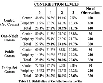
(19) List of Tables Page Table 1.1. Benefits from total contributions in a public account ........ 16 Table 1.2. Payoff to the center given the total contributions of peripheries.................................................................................................... 18 Table 1.3. Payoff to any individual given contributions of her direct neighbors in the circle network................................................................. 22 Table 1.4. Average Contribution Levels in the Star Network.............. 31 Table 1.5. Distribution of Contributions in the Star ............................. 33 Table 1.6. p-values for Binomial Tests on Contributions of Centers . 35 Table 1.7. p-values for Binomial Tests on Contributions of Peripheries ....................................................................................................................... 36 Table 1.8. Difference between Actual and Announced Contributions ....................................................................................................................... 40 Table 1.9. Mapping of Announcements into Contributions for Center Players........................................................................................................... 41 Table 1.10. Mapping of Announcements into Contributions for Peripheries.................................................................................................... 42 Table 1.11. Average Payoffs in the Star Network in each treatment .. 43 Table 1.12. p-values for Mann-Whitney-Wilcoxon test comparing treatments in terms of average earnings in the star network................ 44 Table 1.13. Distribution of Contributions in the Circle........................ 44 Table 1.14. p-values for Binomial Tests on Contributions in the Circle ....................................................................................................................... 46 Table 1.15. Difference between Actual and Announced Contributions ....................................................................................................................... 48 Table 1.16. Mapping of Announcements into Contributions in the Circle (One-neighbor Communication)................................................... 49 Table 2.1. Theoretical predictions and their approximations in the discrete case with 2V = 300...................................................................... 69 Table 2.2. Treatments for Conflict Networks ........................................ 75 Table 2.3. Percentage of subjects’ decisions consistency...................... 80 Table 2.4. Percentage of subjects’ decisions consistency...................... 80 Table 2.5. Percentage of subjects’ decisions consistency...................... 80 Table 2.6. Subjects’ switching behavior................................................... 81 Table 2.7. Subjects’ switching behavior................................................... 82 Table 2.8. Subjects’ switching behavior................................................... 82 Table 2.9. Irrational Subjects..................................................................... 84 Table 2.10. Tests for equilibrium.............................................................. 90 xx.

(20) Table 2.11. Comparing sessions per treatment....................................... 91 Table 2.12. Comparing the independent observations per treatment. 92 Table 2.13. Comparing treatments (via independent observations).... 93 Table 3.1. Lotteries used in the Experiment ........................................ 111 Table 3.2. Combinations of Lotteries offered in Task 3..................... 113 Table 3.3. Possible Responses to Task 3 given PR behavior ............. 117 Table 3.4. Possible Consistent Behavior for first three tasks............. 118 Table 3.5. Overall Possible Consistent Behavior ................................. 120 Table 3.6. Observations on Task 1 and 2 classified by consistent, inconsistent, equal price behavior and total Preference Reversal Rates ..................................................................................................................... 121 Table 3.7. Lottery Specific Preference Reversal Rates ........................ 122 Table 3.8. Percentage of switch decisions in favor of M in Task 4... 123 Table 3.9. Observation number on choice of....................................... 124 Table 3.10. Number of inconsistencies observed in Task 3............... 126 Table 3.11. Predicted choices for Task 3 alone and together with Task 4 ................................................................................................................... 127 Table A. 1. Points for players with label A ........................................... 150 Table A. 2. Points for players with label B........................................... 151. xxi.

(21)

(22) 1. COMMUNICATING PUBLIC GOOD PROVISIONS IN NETWORKS 1.1. Introduction Communicating information to friends, neighbors and colleagues is a common phenomenon. The acquired knowledge on experiences of friends and colleagues helps decisions related to purchase of a new product, investment in a new technology or launching a research project. This is why the analysis of social and economic networks in modeling this phenomenon has recently attained more importance in economics. There is a vast literature that analyzes the effect of exchange of information in innovation. Foster and Rosenzweig (1995) analyze the effects of farmers’ own experimentation along with learning from neighboring farmers on adoption of high-yielding seed varieties newly introduced during “Green Revolution” period in India. Their results show that the profitability of farmers is higher if they have access to experienced neighbors. Yet, they have the propensity to invest less in experimentation of this new technology as their neighbors experiment more, showing their tendency to free-ride on the information obtained by other farmers. Conley and Udry (2001) similarly analyze the role of dissemination of information in the implementation of a new agricultural technology in Ghana. They also show that farmers mimic the successful behavior of neighboring farmers. People get access to new information through their own private research or collecting information from friends or colleagues that 1.

(23) belong to their information neighborhood, i.e. network. Hence, this beneficial information is a public good among individuals that are linked and have a flow of information. Bramoullé and Kranton (2007) take these findings a basis to analyze the production of a costly good that is non-excludable among individuals who are linked to exchange information. within. a. fixed. social. structure.. Keeping. this. social/geographic structure among individuals fixed, they analyze the effect of these network structures on the level and pattern of public good provisions. As their first result, they characterize the Nash level of contributions. They find that for any network structure there are equilibria where some individuals contribute and others free ride. These specialized equilibria follow as a result of efforts being strategic substitutes. As they are faced with multiple equilibria, they later restrict these equilibria to stable ones. The notion of stability used corresponds to the convergence of contribution levels using a Nash adjustment process. They show that a stable Nash equilibrium for any given network structure has to involve some individuals contributing to the public good while others completely free ride. Hence, the first question of this chapter is to see whether equilibrium predictions would hold in a laboratory environment. Since there are multiple equilibria to consider for most of the network structures, experimental results would also resolve the question whether stable or unstable equilibria are observed more often. Yet as Van Huyck, Battalio and Beil (1990) asserts “In economies with multiple equilibria, the rational decision maker … is uncertain which equilibrium strategy other decisions makers will use and …this uncertainty will influence the rational decision-maker’s behavior. Strategic uncertainty arises 2.

(24) even in situations where objectives, feasible strategies, institutions, and equilibrium conventions are completely specified and are common knowledge.” (p.234) Consequently, with the existence of multiple equilibria under this setup, it is quite likely that subjects will face problems of equilibrium selection. Moreover, the characterization of specialized equilibria in simple network structures (like the star and the circle) favors one set of disconnected subjects while disfavoring the other set of disconnected subjects. The resemblance of these specialized equilibria to those observed in a Battle-of-Sexes game is another reason why it is highly susceptible that agents will solve issues of coordination. This provides an incentive to create a mechanism in the design to induce coordination. There is a wide literature that tries to resolve issues of coordination. One approach towards this end has been to introduce cheap talk or a nonbinding communication pre-stage before the actual decision stage. This approach was first experimented by Cooper et al. (1989) and Cooper, DeJong, Forsythe and Ross (1992). They find that in a Battle-of-Sexes game when communication is allowed for only one player, equilibrium play is achieved in 95 percent of the time. Yet, if simultaneous communication is allowed for both players, equilibrium play after equilibrium announcements is observed only 80 percent of the time, but this rate can be improved upon when allowing for communication for more than one round. In line with this literature, this chapter will also introduce a costless and nonbinding pre-communication stage on the intention of play within the described network framework.. 3.

(25) To my knowledge, communication under networks has not been considered experimentally in the earlier literature. Therefore, it will be necessary to further elaborate on the type of communication schemes under a network setup. There are three different mechanisms under consideration. As a first possibility, the communication stage selects a random player to make an announcement on his intention of play. Later this announcement is communicated within the network only to the direct neighbors of the communicator. The results with this additional communication stage demonstrate that this does not provide an improvement on the observed behavior in the laboratory. The second mechanism to test will consider the option of a public announcement. The announcement is again made by a randomly selected player but this time it is communicated to all players in the network. The results under this communication scheme do not improve upon the frequency of observed equilibria play, either. The third communication scheme, instead of picking one player at random to make an announcement, will consider one set of maximal independent players to make an announcement and communicate these announcements only to the direct neighbors of the announcers. Under this mechanism, equilibrium selection is more successful in the star network. The equilibrium in which the center player free rides on the contributions of periphery players is selected over the equilibrium in which peripheries free-ride on the contribution of center player.. 1.2. Literature Theoretical analysis of cheap talk has been considered under private and complete information. Crawford and Sobel (1982) introduced a cheap talk model where a sender communicates with a receiver who 4.

(26) has similar but not identical preferences and is less informed. In this framework,. babbling. equilibria,. where. sender’s. message. is. uninformative and thus ignored by the receiver, always exist. Moreover, even when sender’s message contains at least some information, their results establish multiplicity of equlibria. On the other hand, Farrell (1987, 1988) analyzed the situation where a communication stage on intentions of play precedes an underlying game. In this sequential game with complete information, they demonstrate that communication provides a chance to resolve coordination problems, though not at full efficiency. Farrell and Rabin (1996) classify a message to be highly credible if it is self-signaling and self-committing. A message is self-signaling if the sender truly intends to play his signaled action as he prefers the receiver to best-respond to this signal. On the other hand, a selfcommitting message is one that is part of a Nash equilibrium strategy, creating an incentive for the speaker to fulfill it. On the other hand, Aumann (1990) argues that self-committing messages need not necessarily be credible, i.e. self-enforcing. Charness (2000) to test this disagreement. among. Farrell. (1988). and. Aumann. (1990). experimentally, considers two treatments. In one treatment, senders signal their action and then decide on their actual play, while in the second the order of signaling and decision taking is reversed. In both treatments, receivers take actions after they learn senders’ signals. His results also show that coordination is higher when one-way communication is allowed. However, when actions precede signals, results are not different from those without communication. Clark, Kay and Sefton (2001) also looks into Aumann (1990)’s conjecture 5.

(27) that communication effectiveness will depend on the payoff structure. Their analysis also replicates the fact that communication improves coordination. In the meanwhile, Duffy and Feltovich (2002, 2006) use Farrell and Rabin. (1996)’s. aforementioned. nomenclature.. They. use. communication and observations on past behavior for affecting cooperation. In their earlier work, they show that effectiveness of either of these two depends on the structure of the game under consideration. In their later study, apart from observing signals and past behavior, they also allow for observations on signals from one previous round. This extra treatment allows them to see how subjects weigh these two means of signaling, cheap talk and observations on previous actions. Their additional treatment leads to more cooperation, yet these rates are lower than those when only one of these means is available. Charness and Grosskopf (2004) also study the interaction of communication with observation on previous-round actions. They find that providing information about actions is a factor that substantially increases coordination when there is also the opportunity to communicate about intentions of play. Burton and Sefton (2004) consider two games both with a unique Nash equilibrium. Both games have similar structure of payoffs, except for two outcomes. In one game, equilibrium strategy involves high strategic uncertainty because if coordination is not achieved on the equilibrium outcome, then a negative payoff is probable for either player. Their results show that without communication in the risky game, people play their maximin strategies while equilibrium play is more easily achieved under the less risky game. Yet one introduces 6.

(28) communication to this setup, propensity to coordinate highly increases in the risky game. For a pure coordination game, Parkhurst, Shogren and Bastian (2004) analyze reputation effects in a repeated game (using fixed matching) in comparison to one-shot games (using random matching). For both scenarios they also allow for communication. They show that repetition without preplay communication enhances coordination, yet when preplay communication is allowed, efficiency of cheap talk in terms of coordinating is higher under random matching. Blume and Ortmann (2007) study the effect of preplay communication in median and minimum effort games with multiple Pareto-ranked equilibria – from the framework of Van Huyck et al. (1990) and Van Huyck, Battalio and Beil (1991) – with more than two players. Their results also support that strategic uncertainty, equilibrium selection and coordination is resolved with the help of costless messages on intentions of play. Isaac and Walker (1988) was the first paper to show that face-to-face communication in a voluntary contribution mechanism decreases the free-riding behavior. Afterwards, in a repeated public goods setting Wilson and Sell (1997) analyzed the effect of preplay communication along with information on past behavior (reputation). In contrast to the work of Isaac and Walker (1988), their results on individual level showed that preplay communication hardly matches the actual contribution decisions and hence acts more like cheap talk. Bochet, Page and Putterman (2006) also study possibilities of communication in a voluntary contribution setting. This paper analyzes the effect of different means of communication – face to face, in a chat room and numerical. They also allow for punishment in each possible 7.

(29) communication. scheme.. They. showed. that. face-to-face. communication is the most effective means of communicating in terms of increasing cooperation. Open-ended but anonymous verbal communication in an on-line chat room was also effective but not as much as face-to-face meetings. Moreover, the additional punishment possibility did not significantly alter cooperation levels. As numerical cheap talk did not improve cooperation levels, in a later study, Bochet and Putterman (2009) looked further into the possibility whether making promises on levels of contributions would result better than just announcing intentions of play. They note in this paper that earlier study’s result on numerical cheap talk is mainly due to inter-group differences in the extent to which subjects made false announcements misleading other group members. Although social networks have been of extensive interest and thus thoroughly analyzed through theoretical models, experimental work on networks is quite limited and is still in the path of progress. The line of research that has been under taken in terms of experiments on networks can be summarized in three categories.1 The first set of experiment focuses on the influence of different network structures on equilibrium selection. Keser, Ehrhart and Berninghaus (1998) analyze equilibrium selection in a 2x2 coordination game (with Pareto ranked equilibria) comparing interaction with everybody within the group to a local interaction possibility with direct neighbors in a circle network structure. They show that local interaction allows subjects to coordinate on the risk-dominant. 1. For more detailed discussion on experiments on networks, refer to Kosfeld (2004).. 8.

(30) equilibrium whereas without local interaction coordination the play converges to the payoff-dominant equilibrium.2 Berninghaus, Ehrhart and Keser (2002), on the other hand, analyze equilibrium selection within two different possible setups of local interaction: the circle and the lattice. Even though subjects are not aware of the kind of neighborhood structure they are involved in, their results show that coordination is more likely to focus on the risk-dominant equilibrium under the lattice than in the circle. They explain this observation as a result of the fact that subjects observe less individual decision changes under the circle than in the lattice. Rosenkranz and Weitzel (2008), running an experiment under the setup of Bramoullé and Kranton (2007) mainly focus on the effects of global structures on the behavior on an individual level. They use a within subject design where groups of four subjects, which remains the same until the end of the experiment, take investment decisions under four different network structures. They also test whether there is any coordination on predicted equilibria. They find that this strongly depends on the network structure subjects are assigned to. Their results show that there is only a coordination of 0.4% in the circle and 4.7% in the star network. Hence, results of Rosenkranz and Weitzel (2008) also support my skepticism on coordination failures. Furthermore, in terms of convergence to a stable equilibrium, in the star network, convergence is observed for the equilibria where the center free rides on periphery investments. Additionally, results show Boun My, Willinger and Ziegelmeyer (1999) adapt the setting of Keser et al. (1998) by varying payoffs for the risk dominant and payoff dominant equilibrium in the 2x2 coordination games. As opposed to Keser et al. (1998), their results show that there is no significant difference in terms of convergence to the risk-dominant equilibrium under global and local interaction.. 2. 9.

(31) that convergence under the star network is more stable relative to other three network structures. Rosenkranz and Weitzel (2008) also argue that existence of multiple equlibria for all network structures adds to a strategic uncertainty in the investments of agents, thus they propose that personal risk attitudes may also explain investment decisions. Towards this end, their predictions propose that a riskaverse agent should contribute more, yet their results show to the contrary that relatively risk-averse individuals invest less. The second category of experiments on networks is directed on cooperation. Kirchkamp and Nagel (2007) consider interaction through a repeated prisoner’s dilemma game on a circle. They test to see if cooperation is more likely under this local interaction than in a global interaction setting since players can imitate successful behavior of their neighbors. Their results show that as opposed to the theoretical predictions, cooperation dies out a lot faster under the possibility of local interaction and that players’ own successful strategies reinforce learning more rather than naïve imitation of neighbors’ successful behavior. Cassar (2007) examines the influence of local, random and small-world networks on the sustainability of cooperation and coordination. Results show that though coordination is more likely on the payoff dominant equilibrium in all three networks, play of payoff dominant strategy is observed with significantly more frequency under small-world networks than in the other two structures. As for the prisoner’s dilemma game, it is observed that cooperation is less likely to be achieved in all three networks, particularly with the lowest average cooperation rate in small-world networks. Riedl and Ule (2002) show that cooperation 10.

(32) rates are at a more sustainable rate if players can determine who will belong to their neighborhood of play. Another important line of research on experiments in networks tries to address a crucial question: how networks form. Falk and Kosfeld (2003) test the network formation model of Bala and Goyal (2000), and their results show that subjects are successful in forming strict Nash networks in the 1-way model, but these equilibrium predictions cannot be reproduced in the case of 2-way flow model. Callander and Plott (2005) analyze how networks emerge and what kind of individual decision making processes guide this procedure. Their main results show that emerging networks converge to a pattern that has traits consistent with Nash equilibrium. Rather than using a (Nash) best response model by Bala and Goyal (2000), individuals tend to use simple strategic responses. This paradox between the support for equilibrium in the model but not for the individual decisions leading to the equilibrium is explained through strategy commitment of some agents which may have initiated a means of learning “appropriate” behavior by others. Goeree, Riedl and Ule (2007) consider a network formation game allowing for heterogeneity of agents. They show that stars emerge among heterogeneous agents consistent with equilibrium predictions, which fail to be the case among homogeneous agents. This chapter compared to this strand of literature will also address an equilibrium selection problem, but rather than a 2x2 coordination game, I will use a public goods setup where provisions are strategic substitutes. The equilibria are asymmetric as in a Battle-of-Sexes game, and they are Pareto optimal, but only one is socially optimal. Hence the purpose of this part of the thesis will be resolving coordination 11.

(33) problems and focusing on individual cooperation behavior in the described setup. These issues will be tackled under exogenous networks rather than focusing on formation of these structures. The chapter will be organized as follows. Section 2 will present an introduction to the model by Bramoullé and Kranton (2007). Section 3 will give the details of the design of the experiment along with the theoretical predictions. Section 4 will summarize the results while finally Section 5 will conclude and elaborate on possible further research.. 1.3. Braumollé and Kranton’s Model a) The Model The model of Bramoullé and Kranton (2007), henceforth denoted as BK, considers a group of individuals N = {1, 2,..., n} arranged in a network where benefits within a link flow in both directions. Each individual has to exert an effort level xi, where marginal cost of exerting this effort is assumed to be constant and equal to c. The central assumption in the model is the substitutability of effort levels. Since benefits flow in both directions within a link, effort levels of each individual is a substitute of her neighbors, but not of her neighbors’ neighbors. That is to say, an individual can benefit only from the effort levels of her direct links. Moreover, a neighbor’s effort is also a perfect substitute of one’s own. Thus, with these assumptions an individual i derives benefits from the total of her own and her neighbors’ efforts.. 12.

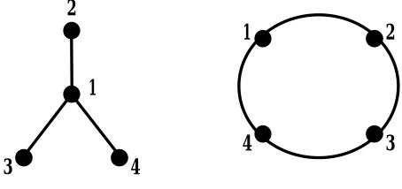
(34) The generic form of the benefit function considered is a strictly concave increasing benefit function b(x) where b(0) = 0. Let x = ( x 1 , x 2 ,..., x n ) denote the effort profile of all individuals. Hence with the earlier assumptions an agent’s benefit is given by  b  xi + . ∑x. j ∈N i. j.   where Ni denotes the set of direct neighbors an . individual i has. Thus, an individual’s payoff from profile x in a given network g is then  U i ( x; g ) = b  x i + . ∑x. j ∈N i. j.   − c ⋅ xi . (1.1). b) Characterization of the Equilibria The characterization of the Nash equilibrium level of efforts goes along in the following manner. Let x* be the effort level at a single node where marginal benefits to an individual is equal to its marginal cost within a link, i.e. b ' ( x∗ ) = c . Then profile x is a Nash equilibrium if and only if for every individual i either (1) x i ≥ x∗ and x i = 0 or (2) x i ≤ x∗ and x i = x∗ − x i where x i is the total effort exerted by i’s neighbors. Hence, an individual exerts effort as long as the total efforts exerted by her neighbours does not exceed x*. If total effort level of her neighbors is less than x*, then the individual will exert effort up to the point that will cover up for this shortage. To elaborate on this characterization further, consider the following two network structures for four individuals given in Figure 1.1 which 13.

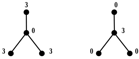
(35) will be the main focus of this experimental study as well. The star network will have one individual in the center with the rest linked to the center. As for the circle network, all individuals will be linked to each other in a recursive manner. 2 1. 2. 4. 3. 1. 3. 4. Figure 1.1. Star and Circle Networks. On the star network, there are two equilibria. The first equilibrium has the center that is linked to all other individuals in the society to exert all the effort, while the rest free rides on center’s efforts. In the other equilibrium, peripheries, individuals linked only to the center and to nobody else, exert all the effort and the center free rides on their effort levels (Figure 1.2). These two equilibria will be referred to as specialized equilibria. In fact, any equilibrium profile where every individual either exerts the maximum amount of effort x* or exerts no effort will be classified as a specialized equilibrium profile. Furthermore, individuals who provide this maximum effort level of x* will be referred to as the specialists. x*. 0. x*. 0. x*. x*. 0. 0. Figure 1.2. Equilibria in the Star Network. 14.

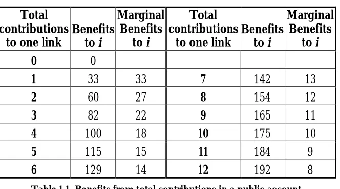
(36) As for the circle there will again be two different equilibria. In one, the effort level will be distributed among all individuals, whereas in the other one a subset of individuals will exert effort; while the rest free rides (Figure 1.3). Hence, in this network structure, there again is a specialized equilibrium where half of the individuals are specialists whereas the other half is non-specialists. x*. 0. 0. x*/3. x*/3. x*. x*/3. x*/3. Figure 1.3. Equilibria in the Circle Network. 1.4. Design of the Experiment a) Experimental Game In this experimental setup, theoretical model proposed and analyzed by BK is implemented. In all treatments, there are groups of four individuals, i.e. n = 4. To keep in line with the model analyzed and to keep the analysis as simple as possible, only the star and circle networks will be analyzed. Moreover, to make the results more comparable with that of a regular public good game, the game will be similar to that of a public goods provision game. In a typical public good experiment, returns from the public good would be linear and same for everyone. Returns from the public good under this setup are no longer linear. On the contrary, as described in BK, they are increasing at a decreasing rate. The returns from total 15.

(37) contributions, which will also be used in the experimental game, are given in Table 1.1. Total Marginal Total Marginal contributions Benefits Benefits contributions Benefits Benefits to one link to i to one link to i to i to i 0 0 1 33 33 7 142 13 2 60 27 8 154 12 3 82 22 9 165 11 4 100 18 10 175 10 5 115 15 11 184 9 6 129 14 12 192 8 Table 1.1. Benefits from total contributions in a public account. As opposed to the total symmetry of a regular public good game, return on the public good in this setup is going to be symmetric only for those players with the same number of neighbors. This difference can be explained in the following manner. In a typical public good experiment, returns of the total contributions are divided equally among all individuals. In this game, this would have been the case if all individuals were in a complete network, where everyone is directly linked to each other. However, within a network structure different from that of the complete network, an individual does not necessarily have a direct link to all others. Thus, in the end, he can only benefit from the contributions of those individuals who he is directly connected to. Hence, most of the time, an individual with more links enjoys more benefits from the total contributions compared to the individuals with fewer direct links. The subjects are given an endowment of 3 tokens in each round. Each subject is assigned to a position in a fixed network structure of a star 16.

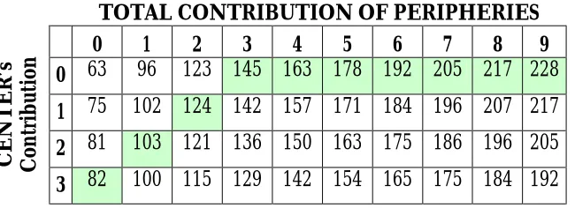
(38) or a circle. They have an option of putting their tokens in a public account or a private account. For every token they keep in their private account, they have a return of 21 per token. Hence, if they choose not to invest anything into the public account, at the end of one round, their payoff will be 63. First note that, as opposed to the direct cost introduced within the theory of BK, in this setup, this cost is introduced implicitly. That is to say, the cost of not investing into the public account is to keep tokens in the private account. Hence, the cost of not investing is c = 21. To put it more formally, let xi be the amount of tokens put in the public account by individual i, and x-i be the amount of tokens invested into the public account by the direct neighbors of i. Then her payoff can be written as, U ( x ; g ) = b ( x i + x − i ) + 21 ⋅ ( 3 − x i ). (1.2). Hence, the first term refers to the benefits of the public good and the second term refers to the benefits of the private account.. b) Predictions for the Star Network Note that the center player, player 1, apart from his own contribution, can get to benefit from a maximum of 9 tokens contributed by his direct neighbors, periphery players – players 2, 3 and 4 (Figure 1.1). Hence, with the mentioned form of payoffs (1.2) and given the total contributions of the peripheries, the payoff to the center is as shown in Table 1.2.3. For a better understanding on calculating the payoffs for each player, please refer to the example in Appendix A. 3. 17.

(39) CENTER’s Contribution. 0. TOTAL CONTRIBUTION OF PERIPHERIES 0 1 2 3 4 5 6 7 8 9 63 96 123 145 163 178 192 205 217 228. 1. 75. 102 124 142 157 171 184 196 207 217. 2. 81. 103 121 136 150 163 175 186 196 205. 3. 82. 100 115 129 142 154 165 175 184 192. Table 1.2. Payoff to the center given the total contributions of peripheries. In this table, highlighted cells correspond to the best responses of the center player. For example, if the total contributions of the center’s periphery neighbors are equal to 0, then his best-reply is to contribute 3. On the other hand, if total contributions of the center’s periphery neighbors are greater than or equal to 3, then his best-reply is to contribute 0. Note also that for a given level of the center’s contribution, as a consequence of the given benefit function he earns more as his neighbors contribute more. However, the relationship in the other direction is not as immediate. Given the total contributions of the peripheries, the center player does not necessarily earn more the more he contributes. More specifically, if peripheries contribute a total of 3 or more tokens, then center player loses as he contributes more. As for the peripheries, since their single neighbor is the center player, maximum number of contributions they can benefit from their single neighbor is equal to 3. Hence to calculate their final payoffs, one needs to consider a smaller version of Table 1.2, so as to say a table that includes only the first four columns. In this manner, the rows labeled from 0 to 3 will correspond to periphery’s own contribution and columns again labeled from 0 to 3 will correspond to contributions of. 18.

(40) their unique neighbor, the center player. Explanations given earlier for Table 1.2 will also apply here. Equilibrium Predictions Now given the number of players, their strategy space, i.e. number of tokens to be invested in each round, and their payoffs, one can elaborate on the predicted equilibria in this game. The equilibrium number of total tokens to be contributed to the public account is determined by the point where the marginal benefit of contributing an extra token to the public project is greater than or equal to the marginal cost of it. In BK, the benefit function under consideration is continuous. Thus, the equilibrium level is the point with marginal benefits exactly equal to the marginal cost. However, in this setup, as a discrete version is considered, the optimal point is the point where marginal cost does not exceed marginal benefit of contributing an extra token. As the marginal cost of not contributing is 21, the highest level of total contributions where this cost does not exceed marginal benefits is at a level of 3 tokens.4 This tells that in the equilibrium every individual has to have access to a total minimum of 3 tokens in the public account they can benefit from. Hence, there are two possible Nash equilibria demonstrated in Figure 1.4. In the figure, the Nash equilibrium on the left will be referred to as the peripherysponsored equilibrium since only peripheries contribute to the public accounts. On the other hand, since it is only the center contributing to the public accounts, the equilibrium on the right will be referred to as the center-sponsored equilibrium.. 3 tokens have a marginal benefit of 22 while 4 tokens have a marginal benefit of 18 according to the benefit table given in Table 1.1.. 4. 19.

(41) 3. 0. 0 3. 3 3. 0. 0. Figure 1.4. Nash Equilibria in the star network under the described game. Efficient contributions The next concern is to determine the efficient level of contributions. First one needs to define the efficient level of contributions. As in BK, a utilitarian approach will be utilized to express the welfare of a profile of contributions x in the fixed network structure g. Hence the total welfare W(x;g) is equal to the sum of payoffs of the individuals: W ( x; g ) = ∑ b ( x i + x i ) − c ∑ x i i ∈N. (1.3). i ∈N. where x i is the sum of contributions of i’s neighbors. Thus, a profile of contributions x is be efficient if and only if there is no other profile x′ such that W(x′;g)> W(x;g). In the first place, welfare of the Nash equilibrium profiles will be determined. In the periphery-sponsored equilibrium, the center benefits from a total of 9 tokens and according to Table 1.2 has a total payoff of 228 whereas each periphery benefits from only 3 tokens and hence each has a payoff of 82. Hence, the total welfare of a peripherysponsored star is W ( periphery-sponsored; star ) = 228 + 3 ⋅ 82 = 474 . On the other hand, in the center-sponsored equilibrium, both the center and the peripheries benefit from a total of 3 tokens. According to Table 1.2, this gives a total payoff of 82 to the center and a total payoff of 145 to each periphery. Hence, total welfare of a center20.

(42) sponsored star is W ( center-sponsored; star ) = 82 + 3 ⋅ 145 = 517 . Thus, the equilibrium level of contributions in the peripherysponsored star is inferior to those in the center-sponsored star in terms of efficiency. Yet, more importantly, the equilibrium level of contributions in the center-sponsored star is not the efficient level of contributions. The efficient level of contributions is where all individuals contribute all of their tokens to the public account. In that case, center benefits from a total of 12 tokens and has a total payoff of 192 according to Table 1.2. As for the peripheries, each benefits from a total of 6 tokens and has a total payoff of 129. Thus, the highest attainable welfare in a star network is given by. Wmax ( x; star ) = 192 + 3 ⋅ 129 = 579 .. c) Predictions for the Circle Network The analysis provided for the star network will be very similar to the one to be made for the circle network. Subjects are again given an endowment of 3 tokens in each round. They again either invest these tokens into a public account or a private account. The benefits are similar to those given in Table 1.1, with the only difference that the maximum level of tokens that a subject can benefit from is 9 instead of the total 12 tokens in the star network. Hence in Table 1.1, one needs to consider only up till the column corresponding to contribution 9 (included).5 As the number of neighbors each subject has is the same, one can summarize the payoffs to each subject in the circle as in Table 1.3: An elaboration on calculation of payoffs in the circle network is provided in Appendix A. 5. 21.

(43) Individual's own Contribution. 0. TOTAL CONTRIBUTIONS OF DIRECT NEIGHBOURS 0 1 2 3 4 5 6 63 96 123 145 163 178 192. 1. 75. 102. 124. 142. 157. 171. 184. 2. 81. 103. 121. 136. 150. 163. 175. 3. 82. 100. 115. 129. 142. 154. 165. Table 1.3. Payoff to any individual given contributions of her direct neighbors in the circle network6. Equilibrium Predictions As the analysis of equilibria provided for the star network does not depend on the network structure, predictions for the circle network will follow in a similar fashion. That is to say, at the equilibrium every subject again has to have access to a minimum of 3 tokens in the public account they can benefit from. This will give way to two different particular equilibria under this structure. Nash equilibrium on the left in Figure 1.5 will be referred to as the distributed equilibrium as all individuals contribute to the public accounts. In comparison, as only a subset of individuals provides contributions to the public account, the equilibrium on the right will be referred to as the specialized equilibrium. 1. 1. 0. 3. 1. 1. 3. 0. Figure 1.5. Nash Equilibria in the circle network under the described game. The highlighted cells again correspond to the best-reply function of a player given the contributions of his neighbors 6. 22.

(44) Efficient Contributions As done with star networks, first an analysis on the welfare of Nash equilibrium profiles will be provided. In the distributed equilibrium profile, every individual puts 1 token and hence enjoys benefits from 3 tokens. Thus, every individual has a final payoff of 124 and the welfare of this profile is W ( distributed; circle ) = 4 ⋅ 124 = 496 . As for the specialized equilibrium, with the existence of individuals who free-ride on the contributions of others, payoffs in this equilibrium profile is uneven compared to the distributed equilibrium. For the specialists, who can only benefit from the 3 tokens they themselves contributed to the public account, their final payoff is 82. As for the non-specialists, who contribute nothing and free ride on the total of 6 tokens contributed by their specialist neighbors, they have a final payoff of 192. Therefore, the welfare of the specialized equilibrium is W (specialized; circle ) = 2 ⋅ 82 + 2 ⋅ 192 = 548 . As a result, for the circle network, the level of contributions in the distributed equilibrium is inferior to those in the specialized equilibrium in terms of efficiency. Similar to the results obtained for the star network; neither of the Nash equilibrium level of contributions is efficient. The efficient level of contributions is where all individuals again contribute all of their tokens to the public account. In that case, every individual gets to benefit from a total of 9 tokens and according to Table 1.3 has a total payoff of 165. Thus, the highest attainable welfare in a circle network is given by Wmax ( x; circle ) = 4 ⋅ 165 = 660 . 23.

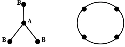
(45) d) Treatments There are three different treatments along with a control treatment. The control treatment essentially mimics the setup of the analyzed theory paper. That is to say it considers a random matching within the star and circle networks. For each network, at the beginning of the experiment, 16 subjects are randomly assigned to groups of four. In the case of the star network, subjects are – again randomly – assigned a label A or B in this network (see Figure 1.6). To avoid further complications in the understanding of the design, subjects maintain their assigned labels throughout the experiment. If they are assigned label A in order to be a center player in the first period, they act as a center player for the rest of the experiment. Same goes through for players with label B, i.e. periphery players. In order to collect statistically independent observations, the random matching is done within cohorts of eight subjects. That is to say, in each session 16 subjects are divided into two cohorts; and, within each cohort of eight, there are two center players (label A) playing against three periphery players (label B) out of the remaining six. Hence, the group of four they are playing in is reassigned at the beginning of each period within this group of eight people.7 As for the circle network of this treatment, like in the star network, subjects are again divided into two cohorts of eight to determine the different groups of four in every period. Note that with the circle network as everybody is in a symmetric situation, it does not really matter what label you get. Hence in the instructions, rather than using labels, subjects are told that they will be benefiting from subjects to their “right” and to their “left” in their assigned. 7. The instructions for this treatment are provided in Appendix A.. 24.

(46) group.8 Once subjects are informed about the structure of the network and their payoffs, they need to take contribution decisions of 0, 1, 2 or 3 for 20 periods. The results from this random matching treatment are used to determine the equilibria played by the subjects without communication. B A B. B Figure 1.6 – Labels used in the experiment. As there are multiple equilibria in both network structures, subjects will face problems of coordination. The approach of introducing cheap talk as a nonbinding communication pre-stage before the actual decision stage as to resolve coordination issues was first experimented by Cooper et al. (1989) and Cooper et al. (1992). Cooper et al. (1992) allowed for two different communication schemes in two different simultaneous coordination games each with a Pareto-dominant equilibrium. In the first communication scheme one player is chosen to announce his intention of playing a certain pure strategy with the knowledge that this announcement is not necessarily binding for the decision stage. This is referred to as one-way communication while the second communication scheme, referred to as. two-way. communication,. involves. both. players. making. simultaneous announcements on their intentions of pure strategy play. 8. The instructions specify to the subjects that individuals to their “left” and “right” are not necessarily sitting next to them but rather they are connected to them through the computer.. 25.

(47) Results show that allowing for one-way communication in a game that is similar to a prisoner’s dilemma game including a dominated strategy for both players increases the frequency of the play of the Paretodominant equilibrium. Yet this does not resolve the coordination problem fully. As for a simple coordination game, results show that allowing for two-way communication, when both players announce the play of the Pareto-dominant equilibrium; actual decisions follow these announcements at a rate of 91 percent. Cooper et al. (1989) used the same methodology this time for a Battle-of-Sexes game. Their results showed one-way communication resulted in equilibrium play 95 percent of the time. In contrast, two-way communication is not as efficient, yet this scheme of communication can be improved upon if players are allowed to communicate with each other in more than one round. Note that in the setup under consideration both network structures have the problem of multiple equilibria. Moreover, the specialized equlibria in each network structure favors a certain subset of players. In the star, the periphery-sponsored equilibrium favors the center player and the center-sponsored equilibrium favors the periphery players. As for the circle structure, the specialized equilibrium favors one set of disconnected subjects while disfavoring the other set of disconnected subjects. This is very similar to the structure of the coordination problem in a Battle-of-Sexes game. This is why it is highly susceptible that agents will face issues of coordination facing an equilibrium selection problem. Hence, taking results from Cooper et al. (1989) and Cooper et al. (1992) into consideration, further treatments in the experimental design will introduce a costless and 26.

(48) non-binding communication stage into the game and hence the described first treatment will act as a control treatment on these communication possibilities. Yet this communication stage needs further elaboration since a network setup is under consideration. There. are. three. different. mechanisms. under. consideration. corresponding to three different treatments: one-neighbor, public and independent set communication. For all communication schemes, there are two sessions – one for each network structure. The subjects’ assignments to positions in the network structure and into groups to form those networks are exactly the same as in the control treatment. In comparison to the control treatment’s sequence of play, prior to their decisions on contribution levels, subjects are informed either to make a non-binding announcement of their intention of play or wait for announcement(s) of selected player(s) according to communication structure. These announcement(s) are communicated to the relevant subjects again in accordance with the communication scheme in hand and are accessible while subjects are making their decisions on how much to contribute. One – Neighbor Communication (One-Neigh Comm) As a first mechanism, one-neighbor communication scheme selects a random player to make an announcement on his intention of play at the communication stage. Later this announcement is communicated within the network only to the direct neighbors of the communicator. In this one-neighbor communication, players who send the announcement and players who receive this announcement are informed that the announcement is non-binding. Hence, any player who is chosen to make an announcement is not forced to follow her 27.

(49) announcement in the decision stage. The most important difference of this announcement. stage. to the. earlier. described. one-way. communication used in the literature is the restriction on the set of players who is going to receive this announcement. As the game under consideration entails networks, the announcement of a player is communicated only to his direct neighbors. In the case of the star network, if a center player is chosen to make an announcement, all periphery players are informed about this announcement. However, if a periphery player is chosen to make an announcement, only the center player learns the announcement while the other peripheries remain uninformed as they do not have a connection with any of the other periphery players. On the other hand, in the circle network, when a randomly chosen player makes an announcement, this announcement is communicated to players to her “right” and to her “left”, but not to the player that is not connected to her. 9 Public Communication (Public Comm) The second mechanism to test considers the option of a public communication, i.e. all players of the network are informed about the announcement. In this mechanism, at the communication stage, again a randomly selected player announces his nonbinding intention of play; and this time this announcement is communicated to all players in the network. Hence, in the case of the star network, if a periphery player is chosen to announce, his announcement is not available only to the center player but also to all other periphery players. In contrast, Instructions for this treatment are also available in Appendix A. In comparison to the first treatment, the only difference appears as an additional communication stage under the section “Your Decision”. 9. 28.

(50) if a center player is chosen to announce in the star, this communication mechanism is equivalent to the first mechanism in the sense that center’s announcement is again communicated to all periphery players. As for the circle network, announcement of the randomly selected player is available not only to his neighbors but also to the third player in the network that he does not have a direct link with. This mechanism is equivalent to the earlier one-way communication proposed by Cooper et al. (1989) since information on intention of play is available to all players irrespective of network structure. Hence it is crucial in terms of comparability to earlier results discussed in the literature. Independent Set Communication (Indep-Set Comm) The last communication scheme to consider, the independent set communication, makes use of a specific structure, maximal independent sets, embedded in networks.10 An independent set of a network is a set of agents such that no two agents who belong to this independent set have a direct link between each other. An independent set is maximal when it is not a proper subset of any other independent set. In a network given a maximal independent set, every agent either belongs to this set or is connected to an agent who belongs to it. The communication scheme to be discussed entails communication across maximal independent sets within the star and the circle. For the star network, there are two independent sets. One is the set of all periphery agents and the other set is the center player alone. Hence, Several results on maximal independent sets have been derived by mathematicians and computer scientists. (see e.g. Gutin (2004)) 10. 29.

(51) in the experiment instead of picking at random a player to make an announcement, the mechanism selects one of these two maximal independent sets. If the center player is chosen, his announcement is available information to all periphery players. Note that, this aspect of the mechanism is again equivalent to the other communication mechanisms discussed. Alternatively, if the maximal independent set of periphery players is chosen, then each of the three periphery players makes an announcement simultaneously which is to be communicated only to the center player. Thus the periphery players do not know what each of them is communicating to the center player. As for the circle network, there are again two disjoint maximal independent sets. Each of the maximal independent sets includes players that have no direct link with each other. More formally, according to Figure 1.1, players 1 and 3 constitute one maximal independent set and players 2 and 4 constitute the other. Hence, if the maximal independent set of players 1 and 3 are selected, they make their announcements which are to be delivered to players 2 and 4, and vice versa in case the maximal independent set of players 2 and 4 are picked to announce. The treatments have been programmed and conducted in Laboratori d’Economia Experimental (LeeX). with the software. z-Tree. (Fischbacher (2007). The participants were undergraduate students from different areas at Universitat Pompeu Fabra. There were two sessions for the control treatment without communication and one session for all other treatments for each considered network structure.. 30.