Essays on Finance and Development
Jacopo Ponticelli
TESI DOCTORAL UPF / ANY 2013
DIRECTOR DE LA TESI
Acknowledgments
My first thanks goes to my advisor Nicola Gennaioli for guiding me through all the stages of this work. His insights and suggestions have been invaluable, and shaped the way I now think about economic questions. He taught me the importance of self-discipline in this job. Most of all, he has been honest with me, as a friend.
I owe a lot to Paula Bustos, Vasco Carvalho and Joachim Voth. They have been great advisors since the beginning of my PhD; I learned from them most of what I know about economics.
I would like to thank Antonio Ciccone, Giacomo Ponzetto, Stephan Litschig, Francesco Caselli, Stefano Rossi and Yanos Zylberberg for their comments and suggestions on the job market paper.
Thanks to Andrei Shleifer for his transparent advice during the job market, and for sharing with me a 1982 Barolo, probably the best wine I will ever taste.
I am indebted to all the people in Brazil who helped me finding the right data, the right questions, and – sometimes – the right bars in Rio de Janeiro and S˜ao Paulo: Claudio Ferraz, Gustavo Gonzaga, Jo˜ao de Mello, Alexandre Samy de Castro, Leonardo Soriano, Eduardo Lundberg. Thanks also to Carlos Lessa, Luis Carlos Pinto and Glaucia Ferreira for their assistance at the IBGE in Rio.
A special thanks goes to Marta Araque, who dealt on my behalf with all the painful real-life administrative obstacles of a PhD student’s life.
Thanks Mapis, Lina and Petri for sharing with me a flat, 100 kilograms of imported pasta, a sailboat, and many other things in the last five years. Thanks Ambro for boarding with me on the wrong flight, and for that Thanksgiving in Washington. Thanks Giulietta and Laura for all the time we spent together inside and outside UPF.
Thanks Tesei for the three years in which we shared office 20.152, and for all your help in the last year. Thanks Felipe for sharing lunches with me al-most daily, and for keeping me updated on the econ gossip. Thanks Bruno, co-author and friend, the man who does not need the mouse. Thanks Commi, Alex, Bruce, Christian, Lien, Philipp, Fabrizio, Stefan, Benedikt, Silvio, Gonc¸alo, Hannes, Jagdish, Ciccio, Miguel and all my fellow PhD students at UPF. Thanks to Michael, you will be missed by all of us.
Abstract
This thesis investigates various aspects of economic development. In the first chapter I study the effect of financial reform on firms. In particular, I study to what extent this effect depends on enforcement’s quality. I find that – when court enforcement works poorly – financial reform increasing creditor protection is in-effective in fostering firm access to credit and productivity. In the second chapter I exploit the adoption of genetically engineered soybean seeds in Brazil to study the effects of agricultural productivity on industrial development. I find that areas more affected by technical change in soy production experienced faster manufac-turing growth due to increased supply of cheap labour and larger credit availabil-ity. In the third chapter I study the relationship between fiscal consolidation and social unrest in Europe using cross-country data between 1919 and 2008. Results show that expenditure cuts are particularly potent in fuelling protests; tax rises have insignificant effects.
Resum
Foreword
My doctoral thesis is a collection of three self-contained essays that study various aspects of economic development, with an emphasis on the role played by financial markets.
In the first chapter I study the impact of a financial reform on firms. Financial reform designed to improve creditor protection is often encouraged as a way to increase credit access for firms, especially in developing countries. I show that when court enforcement works poorly, financial reform is ineffective in fostering both credit access and the productivity of firms. In the empirical analysis, I exploit variation in the quality of court enforcement across Brazilian judicial districts and use a panel of manufacturing firms. I find that, after the introduction of a major pro-creditor bankruptcy reform, firms operating in districts with efficient court enforcement experienced substantially higher increase in capital investment and productivity than firms operating in districts with poor court enforcement. I provide evidence that this effect is due to a higher probability of external funds being used to finance investment in new technologies. To show that the results are not driven by district-level omitted variables, I use an IV strategy based on state laws establishing the geographical boundaries of judicial districts.
In the second chapter, co-authored with Paula Bustos and Bruno Caprettini, we study the effects of agricultural productivity on industrial development. Clas-sical models of structural transformation propose several channels through which productivity growth in agriculture can speed up industrial growth. However – as showed by Matsuyama (1992) – in open economies a comparative advantage in agriculture can slow down industrial growth. We provide direct empirical ev-idence on the impact of agricultural productivity on industrial development by studying the effects of adoption of new agricultural technologies in Brazil. In par-ticular, we use the widespread adoption of genetically engineered soybean seeds as a shock to the productivity of Brazilian agriculture and measure its effects on manufacturing firms. To establish causality, we exploit exogenous differences in soil and weather characteristics across geographical areas leading to a differen-tial impact of the new technology on yields. We find that areas more affected by technical change in soy production experienced faster manufacturing growth. Our findings imply that if technical change is strongly labour saving, increases in agricultural productivity can lead to industrialization even in an open economy.
Contents
List of Figures xiv
List of Tables xvi
1 Court Enforcement and Firm Productivity: Evidence from a Bankruptcy
Reform in Brazil 1
1.1 Introduction . . . 1
1.2 The Brazilian Bankruptcy Reform and the Role of the Judicial System . . . 5
1.2.1 Judicial Efficiency and Firms’ Location . . . 8
1.3 Data on the Brazilian Judiciary . . . 9
1.3.1 Description of Judicial Variables . . . 9
1.3.2 Judicial Variables over Time . . . 11
1.4 A Model of Heterogeneous Firms with Financial Frictions . . . . 12
1.4.1 The Basic Setup . . . 12
1.4.2 Financial Frictions . . . 14
1.4.3 Industry Equilibrium . . . 15
1.4.4 Model Qualitative Predictions . . . 17
1.5 Firm-level Data . . . 18
1.6 Empirics . . . 19
1.6.1 Differences-in-Differences Strategy . . . 20
1.6.2 Differences-in-Differences Results . . . 23
1.6.3 Preliminary Investigation of Aggregate Implications . . . 30
1.6.4 Instrumental Variables Strategy . . . 31
1.7 Conclusions . . . 35
2 Agricultural Productivity and Structural Transformation: Evidence from Brazil 67 2.1 Introduction . . . 67
2.2 Agriculture in Brazil . . . 70
2.4 Empirics . . . 76
2.4.1 Basic Correlations in the Data (OLS) . . . 77
2.4.2 Causality . . . 79
2.4.3 First Stage . . . 81
2.4.4 Reduced Form . . . 82
2.5 Final Remarks . . . 84
3 Austerity and Anarchy: Budget Cuts and Social Unrest in Europe, 1919-2008 105 3.1 Introduction . . . 105
3.2 Data . . . 109
3.3 Results . . . 112
3.3.1 Baseline Results . . . 112
3.3.2 Full Set of Controls, 1970-2007 . . . 113
3.3.3 Results with Exogenous Retrenchment Measures . . . 114
3.3.4 Accounting for Dynamics . . . 115
3.3.5 Institutions and the Sensitivity of Unrest to Austerity . . . 115
3.3.6 Media Penetration . . . 116
3.4 Robustness and Extensions . . . 116
3.4.1 Results by Subcomponent of CHAOS . . . 117
3.4.2 Results by Subperiods . . . 117
3.4.3 Alternative Measure of Unrest . . . 118
3.4.4 Outliers and the Magnitude of Effects in Different Parts of the Distribution . . . 118
3.4.5 Symmetry of Expenditure Increases and Cuts . . . 119
3.4.6 Fiscal Reversals . . . 119
List of Figures
1.1 Recovery Rate in Brazil over time . . . 37
1.2 Trend in Pending Cases per Judge in Brazil . . . 37
1.3 Pending Cases per Judge across Federal States . . . 38
1.4 Comparing Judicial Variables in 2004 and 2009 . . . 38
1.5 State of S˜ao Paulo: Congestion of Civil Courts (upper graph) and Location of Firms (lower graph) . . . 39
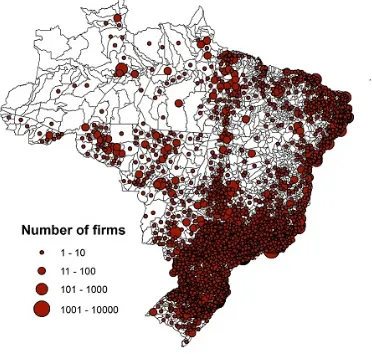
1.6 Location of Firms across Brazil . . . 40
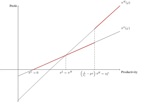
1.7 Profit Functions and Productivity Thresholds . . . 41
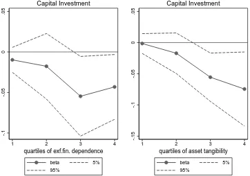
1.8 The Effect of Court Congestion on Investment across Quartiles of Financial Dependence and Asset Tangibility . . . 42
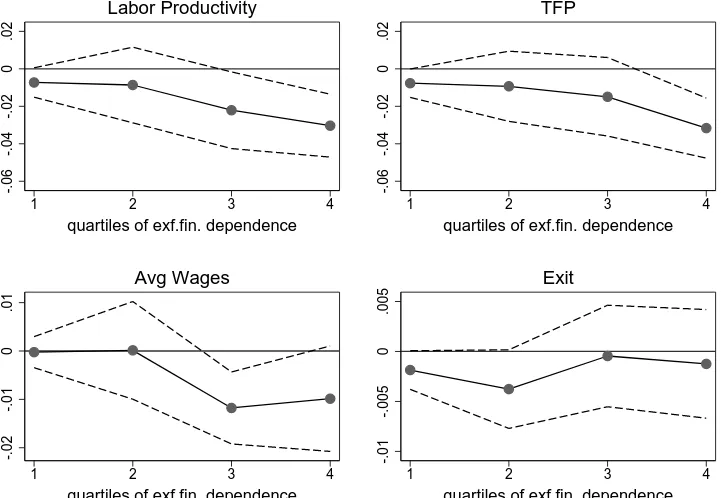
1.9 The Effect of Court Congestion on Firm-Level Outcomes across Quartiles of Financial Dependence . . . 43
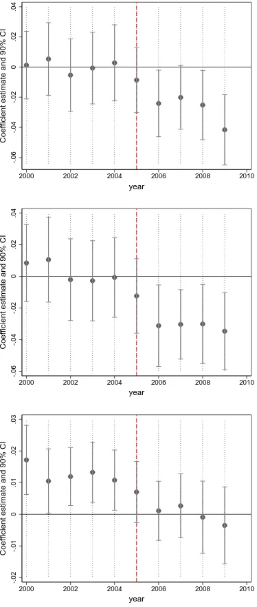
1.10 The Effect of Court Congestion on Labor Productivity, TFP and Wages over Time . . . 44
1.11 Effect of Court Congestion on Labor Productivity over Time and across Industries . . . 45
2.1 Labor Force in Agriculture, Industry and Services, 2002-2011 . . 86
2.2 Area Planted with Soy, 1980-2010 . . . 87
2.3 Labor Force in Soy Production, 2002-2011 . . . 88
2.4 Distribution of Actual Soy Yields across Brazilian Municipalities in 1996 and 2006 . . . 90
2.5 Distribution of Actual Maize Yields across Brazilian Municipali-ties in 1996 and 2006 . . . 90
2.6 Distribution of Actual Sugar Yields across Brazilian Municipali-ties in 1996 and 2006 . . . 91
2.7 Potential Soy Yield Under Low Agricultural Technology . . . 92
2.8 Potential Soy Yield Under Intermediate Agricultural Technology . 93 2.9 Potential Soy Yield Under High Agricultural Technology . . . 94
3.1 Frequency of Incidents and the Scale of Expenditure Cuts . . . . 126 3.2 CHAOS over Time . . . 126 3.3 Changes in Fiscal Variables and GDP Per Capita (% points) . . . 127 3.4 Frequency of Incidents and Economic Growth . . . 127 3.5 Average Change in Expenditure/GDP in Years After Expenditure
List of Tables
1.1 Comparing Brazilian Old Law, New Law and US Bankruptcy Code . . . 46 1.2 Summary Statistics of Judicial Variables, All Courts . . . 47 1.3 Summary Statistics of Judicial Variables, Bankruptcy Courts . . . 47 1.4 Summary Statistics of Firm-level Variables . . . 48 1.5 Comparing Judicial Districts . . . 49 1.6 Firm Investment . . . 50 1.7 Firm Investment, Effects by Financial Dependence and Asset
Tan-gibility (Median) . . . 51 1.8 Firm Investment, Effects by Financial Dependence and Asset
Tan-gibility (Quartiles) . . . 52 1.9 Firm Technological Investment and Access to External Finance . . 53 1.10 Firm Labor Productivity, TFP, Wages and Exit. . . 54 1.11 Firm Labor Productivity, TFP, Wages and Exit, Effects by
Finan-cial Dependence and Asset Tangibility (Quartiles) . . . 55 1.12 Effects by Initial Firm Size . . . 56 1.13 Falsification Test . . . 57 1.14 Average Growth Rates under Different Counterfactual Scenarios . 58 1.15 First Stage . . . 59 1.16 Robustness Check on First Stage . . . 60 1.17 OLS and IV Results Estimated on the Same Sample . . . 61 1.18 Robustness Using Data for Rondonia and Mato Grosso do Sul . . 62 2.1 Land use (millions ha) . . . 89 2.2 Factor Intensity in Brazilian Agriculture: 1996-2006 . . . 96 2.3 Correlations between changes in land by activity: 1996-2006 . . . 97 2.4 Correlation between changes in area reaped with seasonal crops:
1996-2006 . . . 98 2.5 OLS Regressions: Changes in Agricultural Production on Changes
of Area Reaped with Soy and Maize. . . 99 2.6 OLS Regressions: Changes in Industrial Labor Market on Changes
2.7 First stage: changes in area reaped with soy and maize on
poten-tial yield shocks. . . 101
2.8 Reduced form: changes in agricultural production on potential yield shocks. . . 101
2.9 Reduced form results: changes in industrial labor market on po-tential yield shocks. . . 102
3.1 Descriptive Statistics . . . 129
3.2 Cross-correlation Table . . . 130
3.3 Baseline Result . . . 131
3.4 Predicted Number of CHAOS Episodes Under Different Expen-diture Reductions and GDP Growth . . . 132
3.5 Full Set of Controls, 1970-2007 . . . 133
3.6 Exogenous Fiscal Adjustment . . . 134
3.7 Accounting for Dynamics . . . 135
3.8 Institutions and the Sensitivity of Unrest to Austerity . . . 136
3.9 Media Penetration and Unrest . . . 136
3.10 Results by Subcomponent of CHAOS . . . 137
3.11 Results by Subperiods . . . 137
3.12 Alternative Measures of Unrest . . . 138
3.13 CHAOS as a Dichotomous Variable . . . 139
3.14 Unrest, Expenditure Cuts and Growth . . . 139
3.15 Descriptive Statistics, EPCD Dataset . . . 140
3.16 Protest events from EPCD, 1980-1995 . . . 141
Chapter 1
Court Enforcement and Firm
Productivity: Evidence from a
Bankruptcy Reform in Brazil
1.1
Introduction
There is a consensus among economists and policymakers that financial fric-tions are a major barrier to firm investment and thus to economic development (Banerjee and Duflo, 2005; World Bank, 2005). By limiting access to external fi-nance, they can prevent firms from adopting more advanced technologies. In addi-tion, they can hinder the reallocation of capital towards more productive projects, decreasing aggregate productivity (Hsieh and Klenow, 2009).1
Weak protection of creditors is an important source of financial frictions (La Porta et al., 1997; Demirg¨uc¸-Kunt and Maksimovic, 1998; Djankov et al., 2007). In the context of bankruptcy, for example, creditor protection is measured by the effec-tive rights to recover claims from financially distressed firms afforded to credi-tors by national laws and law enforcement institutions (La Porta and L´opez-de Silanes, 2001). In an attempt to improve firms’ access to external finance, emerg-ing economies such as Brazil, China, and Russia have recently introduced new bankruptcy laws increasing the legal protection of creditors. One aspect often overlooked when assessing the potential benefits of these reforms is that, to be ef-fective, they need proper and timely enforcement by courts. Judicial enforcement, however, is seldom well-functioning in many developing countries, where courts in charge of bankruptcy cases are characterized by limited expertise and long
de-1See also: Banerjee and Moll (2010); Buera et al. (2011) and Caselli and Gennaioli (2011).
lays (Dakolias, 1999; Djankov et al., 2008). In such cases, even an otherwise desirable improvement in bankruptcy rules can prove ineffective.
In this paper I assess empirically the extent to which the effects of financial reform depend on the quality of court enforcement. I focus my analysis on Brazil for two reasons. First, it undertook in 2005 a major bankruptcy reform that sub-stantially increased creditors’ chances of recovering their claims when a firm is liquidated. Second, Brazilian judicial districts are highly heterogeneous in terms of efficiency. In some districts, cases are closed within time frames comparable to those in the US. In others, the functioning of courts is undermined by the large number of pending cases. Crucially, Brazilian laws do not allow creditors or firms to choose the district in which to file a bankruptcy case. Therefore, when the new bankruptcy law went into force, the efficiency of local courts became a key determinant of the ability of both creditors and firms to reap the benefits of the reform.
To guide the empirical analysis I propose a simple model of heterogeneous firms in the style of Melitz (2003), in which firms face a fixed cost for technol-ogy adoption. I assume that firms must borrow to pay the fixed cost and that the maximum amount they can borrow depends on two parameters: one captures the strength of creditor protection afforded by national legal rules and is the same for all firms; the other captures the quality of court enforcement and varies across judicial districts. The model has two main qualitative implications when a reform that strengthens creditor protection is introduced. First, firms operating in dis-tricts that have better court enforcement benefit more from the reform in terms of access to external financing, investment in the more advanced technology, and productivity. This effect is heterogeneous across firms: those in the middle of the pre-reform productivity distribution benefit more. Second, because firms in-vesting in the more advanced technology increase their labor demand, the reform increases wages relatively more in districts that have better court enforcement. Higher wages drive out of the market the least productive firms and reallocate labor to the more productive ones.
2009.2
The baseline diff-in-diff results are consistent with the predictions of my model. First, firms operating in (one standard deviation) less congested judicial districts experience higher increase in capital investment (4.4%) and firm productivity (1.9%) after the introduction of the reform. The size of these effects is substantial: a one standard deviation in court congestion explains approximately 20% of the average increase in capital investment and 10% of the average increase in total factor productivity (TFP) in the years under study.3 I further show that these ef-fects correlate with a higher probability of external funds being used to finance investment in new technologies. Consistent with the model, most of the effect of court congestion on investment and productivity is driven by middle-to-large firms. Furthermore, I find a larger increase in average wages in districts with less congested courts. Finally, in these districts, small firms are more likely to exit the market.
Brazilian laws establish that bankruptcy cases must be filed in the judicial district where the headquarters of the firm is located. A first challenge to my identification strategy is that firms might initially decide where to locate their headquarters based on the quality of court enforcement. I tackle firm selection by showing that court enforcement is not a significant determinant of firm loca-tion in the pre-reform period. A second challenge involves the fact that districts with better enforcement might also have other desirable characteristics driving the main results. I show that my diff-in-diff results are robust to controlling for initial conditions at the judicial district level such as average household income, number of banking agencies, and population. Exploiting the panel dimension of the firm-level dataset, I also verify that the diff-in-diff results are not driven by different background trends across districts.
To address endogeneity I also propose an instrumental variable (IV) strategy that corroborates the diff-in-diff results. The IV strategy is based on state laws that, starting from the 1970s, established minimum population size requirements for municipalities to become independent judicial districts.4 Crucially, jurisdiction over municipalities below these minimum requirements was assigned to the courts of a territorially contiguous municipality that met the requirements. I construct the instrument as follows. First, I restrict my sample to those municipalities that,
2The surveys are: the Annual Industrial Survey (PIA), from which I use yearly data from 2000
to 2009, and the Survey of Technological Innovation (PINTEC), that is produced every 2/3 years and for which I use the waves of 2000, 2003, 2005 and 2008.
3These are percentages of the average increase in capital investment and TFP observed at the
firm level between the pre-reform years (2003–2005) and the post-reform years (2006–2009), respectively, 23% and 19.8%.
4State laws on judicial organization in Brazil have been used also by Litschig and Zamboni
given their population, could have been an independent judicial district. Second, I compute for each of these municipalities the total population of their neighboring municipalities below the minimum requirements at the time the state laws were introduced. This is a measure of the initial extra jurisdiction assigned to judges by state laws that only depends on characteristics of neighboring municipalities. I use this as an instrument for current court congestion. Because the population of a subsample of neighbors can also determine firm-level outcomes through market size effects, I control for the total population of all neighboring municipalities, regardless of whether they were above or below the minimum requirements.
Existing work on the relation between legal protection of creditors and judicial efficiency has exploited cross-country differences (Djankov et al., 2003; Claessens and Klapper, 2005; Safavian and Sharma, 2007). These differences are likely to correlate with other unobserved country characteristics, such as the investment climate or the level of political accountability, that also affect financial develop-ment and the other outcomes under study. Research work using within-country data – which mostly relies on across-state variation – has focused on the effect of enforcement quality and not on its interaction with financial reform. For example, using loan-level data from a large Indian bank, Visaria (2009) finds that the intro-duction of specialized tribunals increases loan repayment and lowers the cost of credit for firms.5 Lilienfeld-Toal et al. (2012) use Indian data to show theoretically
and empirically that when credit supply is inelastic, the existence of specialized courts reduces access to credit for small firms and expands it for big ones.6 An-other stream of empirical literature studies the aggregate effects of bankruptcy reform, but without focusing on the role of the judiciary in shaping these effects. For example, Araujo et al. (2012) analyze the effect of the Brazilian bankruptcy law reform on the financing decisions of publicly traded Brazilian firms using as control group publicly traded firms in neighboring countries.7 The main
contri-bution of my paper to the existing literature is that, to the best of my knowledge, I provide the first empirical evidence on the interaction between financial reform — in particular, bankruptcy reform — and court enforcement at the micro level.
On the theoretical side, several papers in the bankruptcy literature tackle the
5I do not find that firms that operates in districts with bankruptcy courts experienced a larger
increase in investment and productivity in the aftermath of the reform. A possible explanation is that, in comparison to India, specialized courts in Brazil tend to be more congested than normal civil courts (see also De Castro (2009)).
6Other papers using within-country variation in judicial variables are Chemin (2012), which
studies the impact of judicial reform on the lending and investment behavior of small firms in India; Jappelli et al. (2005), which exploits variation across Italian judicial districts to establish a relation between judicial efficiency and bank lending; and Laeven and Woodruff (2007), which studies how the quality of the legal system at the state level affects firm size in Mexico.
7See also: Gamboa-Cavazos and Schneider (2007) for Mexico and Rodano et al. (2011) for
judicial system’s role in shaping bankruptcy outcomes – for better or worse. Gen-naioli (2012) proposes a model in which the ability of courts to properly enforce contracts depends on their ability to verify actual states of the world, e.g. the return of a given project. When these states are not easily verifiable, courts’ veri-fication generates enforcement risk in financial transactions. Gennaioli and Rossi (2010) show how judicial discretion can lead to an efficient resolution of financial distress, but only in a reorganization framework that offers strong creditor pro-tections. Ayotte and Yun (2009) stress the potential negative effects of judicial discretion when judges are not trained or do not have the necessary experience to effectively run the bankruptcy procedure. Ichino et al. (2003) show that judi-cial enforcement can lead to different outcomes in similar firing cases made under the same national laws, especially when such laws leave a wide range of possible interpretations to judges.
The rest of the paper is organized as follows. In section 1.2 I describe the Brazilian bankruptcy reform and how the efficiency of the judicial system influ-enced its impact on creditors. Section 1.3 presents the data on the Brazilian ju-diciary. In section 1.4, I present a model of heterogeneous firms which delivers qualitative predictions on firm level outcomes. Section 1.5 describes the firm-level data used to test these predictions. In section 2.4, I present the identification strategy and the empirical results.
1.2
The Brazilian Bankruptcy Reform and the Role
of the Judicial System
Until 2005 bankruptcy in Brazil was administered under Law 7,661, in force since 1945 (hereafter the “old law”). The old law was particularly unfavorable towards secured creditors, banks that provide loans guaranteed by collateral. In most developed countries, including the US, secured creditors have the right to repossess the collateral when a firm defaults on its debt. In Brazil, instead, the collateral proceeds are pooled together with the rest of the firm’s assets and then used to repay creditors in an order established by law. Under this framework, secured creditors were put at a strong disadvantage by two characteristics of the old liquidation procedure:8 successor liability and first priority given to labor and tax claims.
Successor liability implied that, in liquidation, the debts of a firm were passed on to the purchasers of the firm or of its business units. This dampened the value of financially distressed firms, which had to be discounted for the known debt,
8I focus here on the liquidation procedure, representing on average 97% of bankruptcy
the costs of due diligence, and the risk associated with possible unknown debts. Successor liability did not apply when firm assets were sold separately instead of jointly (e.g., a single loom versus an entire textile plant), creating strong incentives to sell assets piecemeal, which further reduced the proceeds from liquidation.
The second characteristic of the old law was that labor and tax claims had first priority in the order of repayment. Only afterwards came secured creditors. The absolute priority rule required that labor and tax claims had to be paid off in full before anything was given to secured creditors. As a consequence, their probability of recovery was minimal once an official bankruptcy procedure was initiated.9
In June 2005 Brazil introduced a new bankruptcy law (Law 11,101) inspired by chapters 7 and 11 of the US bankruptcy code. The conflict of interest between the fiscal authority and the banking sector – the former interested in maintaining its priority on secured creditors, the latter pushing to reverse it – lead to high uncertainty about the wording of the final draft. In this sense, the exact content of the new rules could hardly be anticipated until the end of 2004.10
One of the objectives of the new law was to increase creditors’ recovery. To this end, the new law introduced several important innovations (see Table 1.1 for a detailed description). In this paper I focus on three of them: (i) removal of successor liability when selling business units or the entire firm as a going con-cern, (ii) introduction of a cap of 150 monthly minimum wages11 per employee
on labor claims, and (iii) priority of secured creditors’ claims over tax claims. The first point states that claims remain liabilities of the debtor and are no longer passed on to the purchasers (art. 141). This increased the value of distressed firms when sold in full or by business units. The second point was introduced to avoid fraud, because it was not uncommon for the management personnel of firms in financial distress to fix unreasonably high salaries for themselves before entering into bankruptcy, knowing they would enjoy the same priority as their employees. The third point was introduced to increase the protection of banks – those pro-viding credit guaranteed by collateral. If the first point increased the potential value of firms in financial distress – and therefore the recovery rate of creditors – the second and third points reduced uncertainty about the bankruptcy outcome
9This had the additional negative effect of lowering the incentive for secured creditors to
bring financially distressed firms to court in the first place. They delayed the filing for a firm’s bankruptcy as long as possible, and only did so when the firm’s debt situation was already unsus-tainable. Thus, firms entering official bankruptcy were usually in particularly bad shape, reducing even further the probability that creditors would recover any of their claims.
10The final wording of the law was only revealed at the end of 2004 after several passages
through the two houses. The new law was applicable only to bankruptcy cases filed after it entered in force.
for secured creditors, allowing them to evaluate ex-ante their likely recovery on each loan. In fact, under the new law, a bank can estimate the present discounted value of the collateral necessary to guarantee full recovery if the firm were to go bankrupt.12
A survey of legal professionals promoted by the World Bank for the Doing Business Database suggests that the average recovery rate – expressed in cents per claimed dollar that creditors (be they workers, the tax authority, or banks) are able to recover from an insolvent firm – was 0.2 cents on the dollar in Brazil at the time the reform was passed. This is a negligible fraction of outstanding claims when compared, for the same year, with the US (80.2), India (12.8), and China (31.5). Figure 1.1 shows the pattern of the recovery rate in Brazil from 2004 to 2012. According to the World Bank, the recovery rate had a discrete jump about two years after the introduction of the reform, going from 0.4 in 2006 to 12.1 cents on the dollar in 2007. This pattern is consistent with the legal changes introduced by the bankruptcy reform, especially the removal of successor liability, which aimed to increase the value of firms sold in bankruptcy. However, the level attained is still far from that of the US. Table 1.1 compares the old Brazilian law, the new law and the US law. It shows how the gap with the US in terms of legal rules has been drastically reduced with the introduction of the new law. Why is therefore the gap in terms of recovery rate still so wide?13 Part of the explanation lies in the efficiency of the judicial system. In the US, bankruptcy cases are closed in an average of 1.5 years. My data show that in Brazil, this take between 5 and 6 years.
Brazil is an ideal laboratory to study how much the efficiency of the judicial system can affect the impact of a major legal reform. Brazilian laws establish that bankruptcy cases must be filed in the civil court that serves the area where the debtor’s headquarters is located. Unlike the US — where forum shopping is a diffuse practice, in particular for big reorganization cases (e.g., Eisenberg and LoPucki, 1999) — Brazilian judges tend to consider a firm’s headquarters to be the location where most of the economic activity of the firm takes place.14 This
12As an example, take a firm with 10 employees asking for a loan worth US$ 200,000. The bank
knows there are, at maximum, labor claims worth in total US$ 200,000 (assuming US$ 20,000 per employee) with priority over its own claim in case of default. As a consequence, for a loan worth US$ 200,000, a bank will ask a collateral worth at least US$ 400,000 at the time of maturity.
13One option is that it simply takes some time to digest the new rules and that Brazil will
eventually catch up with the US in terms of efficiency of its bankruptcy process. But the data seems to tell a different story. After the reform the recovery rate stabilized at around 17 cents on the dollar, and it is not in an increasing pattern.
14This practice became widespread after cases such as the one of Grupo Frigor`ıfico Arantes, a
definition of a firm’s headquarters makes the relocation for judicial purposes an extremely expensive process. In addition, under the old bankruptcy regime, the negligible recovery rate of creditors made the costs associated with relocation outweigh the benefits of a more favorable judicial environment. Finally, the vast majority of bankruptcy cases in Brazil are cases of liquidation, where the man-agement has no power to choose the bankruptcy venue.
Second, Brazil is an ideal laboratory because it offers vast cross-sectional vari-ation in judicial variables that can be exploited. Brazil is divided into more than 2,500 judicial districts, and each district has at least one court of first instance that handles civil cases, including bankruptcy.15 Moreover, courts proceed at vastly
different speeds across the country. Judicial data presented in this paper suggests that closing a civil case can take less than a year in some districts, and up to 30 years in others.
Slow courts are likely to have had a negative effect on the incentive to lend under both the old and the new law. The key assumption here is that for secured creditors (that in the pre-reform period expected to recover nothing regardless of court speed), the quality of court enforcement became a critical factor in deter-mining their chances of recovery only in the post-reform period.16
1.2.1
Judicial Efficiency and Firms’ Location
Is the efficiency of civil courts a key determinant in where firms choose to initially establish their headquarters? Even if forum shopping is not allowed or is extremely costly in Brazil, firms might decide to establish their headquarters in districts with better enforcement because, for example, in such districts it is easier to get a line of credit.17 This is a potentially important selection problem: if all
firms tend to locate where courts are more efficient, then the aggregate costs of judicial inefficiencies are negligible. As a first check to the data, in the empirical section I show that judicial districts characterized by different degrees of court ef-ficiency are not systematically different in terms of the number of manufacturing firms registered under their jurisdiction in the pre-reform period. If anything,
dis-capital Cuiab´a does not even have a permanent judge.
15Bankruptcy cases are a small fraction of the cases for which civil courts function as courts of
first instance. They usually share the judge’s desk with tax disputes, car accidents, divorce cases etc.
16The crucial role of the judiciary in the enforcement of the new law has been highlighted by
academics (Araujo and Funchal (2005)), practitioners (Felsberg et al. (2006)), and the Brazilian Central Bank (Fachada et al. (2003)).
17The relationship between firm location and court enforcement quality is not straightforward:
tricts where courts are more congested register a higher number of manufacturing firms in 2000, the initial year. I also show that from 2000 to 2009 there is very little firm mobility across districts: about 1.5% of firms changed judicial districts every year on average. As an additional robustness test, in the empirical section I show that the main results hold if I restrict the sample to those firms that did not change location after the introduction of the bankruptcy reform, or to single-plant firms, those for which the possibility of forum-shopping would be more costly.
1.3
Data on the Brazilian Judiciary
In section 1.2 I argued that the new law made court speed a key determinant of creditors’ and firms’ ability to reap the benefits of the reform. In this section, I document the vast cross-sectional variation (subsection 1.3.1) and the high per-sistence over time (subsection 1.3.2) of court congestion across Brazilian judicial districts.
1.3.1
Description of Judicial Variables
Data on the Brazilian judiciary come fromJustic¸a Aberta, a database produced by the Brazilian National Justice Council (CNJ).18 The dataset covers all courts
and judges working in the Brazilian judiciary, and the data are collected monthly through a standard questionnaire filled out by the judges or the administrative staff of each court. Data at the court level19 include the type of court (civil, criminal,
etc.), the year of creation, the administrative staff available, the number of cases pending at the end of each month, the number of new cases filed per month, the number of hearings per month, and the number of cases sent for review to higher courts per month. Data at the judge level include, for each court in which the judge worked during the last month, the number of days worked, the number of cases closed and the number of hearings. The database allows me to match judges with courts, and courts with judicial districts. Brazil is divided in 2,738 judicial districts, which are the smallest administrative division of the judiciary. A judicial district can correspond to a single municipality, or can encompass a group of them. Using official documentation provided by state tribunals, I map each judicial district to the municipalities it includes.20
18All judicial data used in this paper can be downloaded from www.cnj.jus.br.
19Data is available for both courts of first and second instance. I focus my analysis on courts of
first instance.
20Because the geographical identifier for Brazilian firms is the municipality in which they
The measure of court enforcement quality I am interested in is court speed in closing bankruptcy cases. Because data on case length by type of case is not available, I follow the existing literature on judicial productivity (Dakolias, 1999) and use as a proxy the backlog per judge, defined as the number of pending cases in a court at the beginning of the year over the number of judges working in that court over the year.21 I compute this measure at the judicial district level using
only civil courts, those that deal with bankruptcy cases. For those judicial districts that have two or more civil courts, I take a weighted average of court congestion, using as weights the total number of open cases in each court.
Finally, 12 judicial districts22have courts that specialize in bankruptcy cases. Where these courts exist, the judicial district is assigned their measure of court congestion.23 Out of the 8,621 courts of first instance initially recorded in the
database (which include not just civil courts, but also criminal courts and courts specialized in various types of cases, from tax evasion to child protection), I select 4,126 civil courts and the corresponding 5,276 judges that deal with bankruptcy cases.24 After taking averages across courts within districts where more than one court handles bankruptcy cases, I am left with data on 2,507 judicial districts, 92% of all of those existing in Brazil.25
Table 1.2 shows descriptive statistics of the main judicial variables. The unit of observation is the judicial district, and all data refers to 2009. Each judicial district in Brazil has, on average, 1.6 civil courts, and each court has an average of 2.2 judges and 12.7 administrative staff members. The congestion rate is the sum of pending and new cases filed over a year, divided by resolved cases, and it can also be interpreted as the number of years necessary to solve all currently open cases at the current pace. Notice that the average congestion rate is 5.4, suggesting that at the current pace it will take, on average, slightly more than five years to
21Unfortunately, the data do not allow me to observe the work practice of judges. In particular,
I can not observe whether judges start working on cases in the order they enter into the court or whether they give priority to new cases. Coviello et al. (2011) show that work practices, and in particular how workers deal with pending tasks, can influence worker’s productivity. Coviello et al. (2012) apply this reasoning to the case of Italian judges and find that “task juggling” negatively affects the speed at which they close cases.
22These are Belo Horizonte, Brasilia, Campo Grande, Curitiba, Fortaleza, Juiz de Fora, Novo
Hamburgo, Porto Alegre, Rio de Janeiro, S˜ao Paulo, Uberaba, and Vitoria.
23Specialized courts employ judges with a sound understanding of bankruptcy procedures. They
might play a different role independently of their productivity. I explore the role of courts special-ized in bankruptcy more extensively in the empirical section.
24I can classify these courts by type as follows: 2,306 civil courts, 1,797 general courts (“vara
unica”, these are the only tribunal available in these judicial districts and deal with all types of cases), and 23 courts specialized in bankruptcy law.
25The missing 8% comprises mostly judicial districts located in remote areas, e.g., the
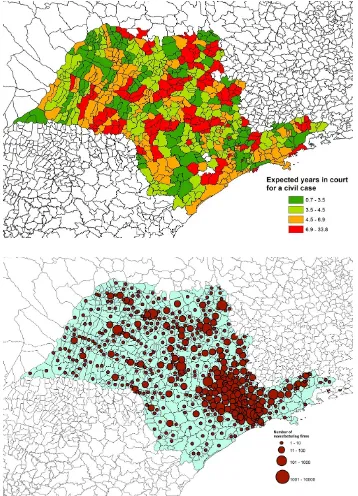
close a bankruptcy case filed this year in a Brazilian court. Notice also the large heterogeneity in the cross-section. The congestion rate has a standard deviation of 4.9 and ranges from 0.6 to more than 30, suggesting that some judicial districts, judicial productivity is close to that of US standards (even though some of these outliers are remote places with few cases), while in others it can take more than 30 years for a case entering the court today to reach resolution. Figure 1.5 (upper graph) show a map of the state of S˜ao Paulo where judicial districts are separated in four quartiles of court congestion rate.
Interestingly, courts specialized in bankruptcy law (descriptive statistics re-ported in Table 1.3) tend to be slower in case resolution than normal civil courts and to have a higher rate of appeal, i.e. more cases sent to higher courts for re-vision. The average congestion rate of bankruptcy courts is 8, and their initial backlog per judge is more than 2000 cases larger than that of all other courts. In addition, their appeal rate is on average 20%, meaning that one case out of five is sent to higher courts for revision, while in normal courts just one case out of ten is. This is only suggestive evidence, since I can not observe whether different types of cases proceed at different speed within civil courts.
1.3.2
Judicial Variables over Time
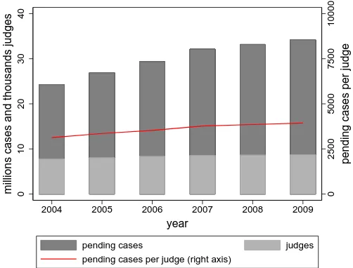
How has judicial congestion behaved over time in Brazil? Has it been affected by the implementation of the bankruptcy reform? I check for trends at the state level, a higher level of aggregation than the judicial district, using data starting from 2004 (the first available year for data at state level). Figure 1.2 displays the strong stability of the ratio of pending cases per judge between 2004 and 2008 in Brazil as a whole. Figure 1.3 shows the same variable in four Brazilian states, one per quartile of the distribution of court congestion at the state level: S˜ao Paulo, Rio Grande do Sul, Rondonia, and Paran´a. Notice the large heterogeneity in the level of court congestion across states and its persistence over time within each state.
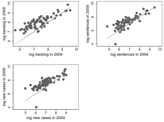
tribunals starting from 2004.26 Figure 1.4 shows the scatterplots of the number of pending cases, new cases, and sentences (expressed in logs) for 2004 and 2009 for all judicial districts in these two states. Even though these states constitute a small fraction (5%) of all judicial districts, the figure suggests that there is little variation over time in the judicial variables even at this finer level.27 More
impor-tantly, in section 2.4 I verify that i) the main results of the paper hold when using only judicial data from these two states and ii) using judicial data from 2004 or 2009 gives very similar coefficients on the main outcome variables. In the OLS regressions, I therefore use the cross-sectional variation in court congestion at the judicial district level in 2009 as a proxy of its pre-reform level. In section 1.6.4, I then propose an instrument that is predetermined with respect to the 2005 reform for all judicial districts.
1.4
A Model of Heterogeneous Firms with Financial
Frictions
In section 1.2 I described a major financial reform introduced in Brazil in 2005 that, by increasing secured creditors chances of recovery, should have increased their ex-ante lending incentives. In section 1.3 I showed empirical evidence on the quality of court enforcement: data suggests that it is vastly heterogeneous across Brazilian judicial districts and relatively stable over time. This section provides a conceptual framework for understanding the effects of bankruptcy reform on two sets of firm-level outcomes: those directly affected by the reform, such as firm access to external finance and investment, and those indirectly affected by the reform, such as technological upgrade, productivity, wages, and exit. To this end, I present a simple model of heterogeneous firms in which access to credit affects firms’ technological upgrade through a fixed cost of innovation that can not be financed with internal funds. My theoretical framework builds on Melitz (2003) and Bustos (2011), by adding financial frictions that depend on both na-tional bankruptcy rules and efficiency of local courts.
1.4.1
The Basic Setup
There are two dimensions of heterogeneity across firms, both exogenously determined. The first is each firm’s initial productivity level (ϕ). This can be thought of as the quality of the management or the potential of the project that each firm wants to carry out. The second dimension of heterogeneity is the location in
26The original documentation can be downloaded from www.tjro.jus.br and www.tjms.jus.br.
which each firm operates, described here as a judicial district. I assume that, at least in the short term, there are infinite moving costs across judicial districts for both firms and workers.
The consumer utility function takes the C.E.S. form:U =Rω∈Ωy(ω)σ−σ1dω
σσ−1
, where σ > 1 is the elasticity of substitution across different varieties (identi-fied byω). Maximizing this utility function subject to the expenditure constraint
R
ω∈Ωp(ω)y(ω)dω=E, whereEis the aggregate spending in this economy, gives
the demand for a single variety:
y(ω) = p(ω) P −σ E P (1.1)
whereP = Rω∈Ωp(ω)1−σdω
1−1σ
is the aggregate price index.
Each firm produces one of these different varieties in a single industry under increasing returns to scale. Labor is the only factor of production, and judicial-district-specific wages are the num´eraire. Entrant firms draw their own productiv-ityϕfrom a known distribution G(ϕ). Entry is disciplined by fixed set-up costs (fe), expressed in terms of labor, that guarantee a finite number of entrants. Once
firms observe their productivity, they decide whether to stay and produce or to exit the market. In addition, in every period there is an exogenous probability of exite
for an unexpected bad shock. Those firms that stay in the market can produce their varieties using a low technology (L), which is a basic technology that features a relatively low fixed initial cost (f) and a constant variable cost (both expressed in terms of labor). They also have the option to switch to a high technology (H) that reduces their marginal labor cost but has a larger fixed cost. Production under different technologies is described by the following total cost functions (T C):
T C =
(
f+ ϕy if technology =L
ηf +γϕy if technology =H(η, γ >1)
Firm profits are a positive function of productivity:
π =
(
(1−τ)¯πL−f if technology =L (1−τ)¯πH −ηf if technology =H
In this equation,π¯stands for firm operating profits net of variable labor costs. It is equal to(ϕγ)σ−1 σ−1
σ
σ−1 E
σP
σ−1 in case the firm operates with theH
tech-nology. It is equal to(ϕ)σ−1 σ−1
σ
σ−1 E
σP
σ−1in case the firm operates with theL
There is a unique productivity cutoff (ϕ∗) above which firms find it profitable to stay in the market. The cutoff is determined by the zero profit condition for a firm using the low technology:πL(ϕ∗) = 0. There is another unique productivity cutoff (ϕh) above which firms find it profitable to switch to the high technology
(pinned down byπH(ϕh) = πL(ϕh)).
I assume that the high-technology fixed cost can not be financed using internal funds, so that firms that find it profitable to switch to the high technology — those whose productivity is such thatϕ > ϕh — need to borrow from financial
intermediaries.
1.4.2
Financial Frictions
Financial intermediaries will lend to firms if they are guaranteed to recover their claims in case of default. This implies that financial intermediaries are will-ing to lendbas long as:
(1−pτ)¯πH −(1 +r)b>
1− 1
ψj
¯
πH (1.2)
The left-hand side of equation 1.2 represents firm profits after repaying taxes and the privately contracted debtb (on which it pays an interest rate r). The pa-rameterpcaptures how pro-investors the bankruptcy rules are. The higher isp, the lower the share of firm profits that is appropriable by financial intermediaries — either because there are classes of creditors with priority over them (in this case, the government) or because the bankruptcy rules (such as those on successor lia-bility) do not preserve the value of the firm in liquidation. A value ofpclose to 1 might capture the fact that the government has first priority over financial inter-mediaries or that the bankruptcy procedure is particularly inefficient in preserving the value of liquidated assets, or a combination of these factors.
The right-hand side of equation 1.2 represents the share of firm value28 that
can not be seized by courts.29 The share ψ1
j is the judicial-district-level measure of the quality of court enforcement, which is assumed to be a negative function of
ψj, the parameter capturing court congestion. One can think ofψj as the discount factor for the number of years that a bankruptcy case stays in court in a given district, and of π¯ψH
j as the resulting value of a firm at the end of the bankruptcy
28Operating profits net of variable labor costs before paying debt due to private financial
inter-mediaries. Remember that in this setup all firms that want to borrow find profitable to switch to the high technology
29The ability of courts to seize defaulting firm’s assets is a key parameter in several
process. I assume that there are j = 1, ...J judicial districts in the country and thatψj varies across districts.
Under these assumptions, financial intermediaries will lend b as long as firm profits in the case of repayment are larger that the share of the firm value that can not be seized by courts in the case of default. The maximum amount of debt that a firm can obtain from financial institutions is therefore pinned down by equation 1.2 solved with equality. Whenp > 0and assuming for simplicity thatr = 0, this is given by:
max{b}=
1 ψj −pτ ¯ πH,0
(1.3) Equation 1.3 shows the complementary role played in this model by the two frictions that constrain firm borrowing: legal rules (p) and enforcement quality (ψj). Notice also how the two frictions operate at different geographical
dimen-sions:pis the same for all judicial districts, whileψj varies across districts.
To adopt the high technology, firms must borrow at least enough to pay the fixed cost ηf. Firms are financially unconstrained as long as max{b} > ηf.30
All firms whose productivity is such thatmax{b}< ηf (but high enough that the adoption of the new technology is a profitable option) are instead financially con-strained.31 To find the productivity cutoff to be unconstrained (ϕu) I setmax{b}= ηf. Figure 1.7 shows in red the optimal technological choice as a function of firm productivity.
1.4.3
Industry Equilibrium
The industry equilibrium is pinned down by the zero profit condition and the free entry condition. Free entry requires the fixed entry cost to be equal to the present value of expected profits, discounted by the per-period probability of exit due to a bad shock (e):
fe = [1−G(ϕ∗)] ˜ π
e (1.4)
where[1−G(ϕ∗)]is the probability of survival, i.e., the probability of drawing a productivity higher than the exit cutoff productivity (ϕ∗).
When financial frictions play a role, expected profits are defined as follows:
˜
π=puπ˜u+pcπ˜c (1.5)
30In this case, the value of the firm in the case of default is large enough to repay all debtors,
because ¯πψH
j >τ¯π
H+ηf.
31In the extreme case in whichτ
> ψ1j, financial intermediaries will never recover anything at
wherepu is the probability of an active firm being productive enough to be
un-constrained, whilepc is the probability of being constrained (both conditional on
being active). Formally, pu = 11−−GG((ϕϕu∗)), and pc =
G(ϕu)−G(ϕ∗)
1−G(ϕ∗) . If the firm is
unconstrained, then its expected profits are given by:
˜
πu =
Z ϕh
ϕ∗
πL(ϕ) g(ϕ)
1−G(ϕ∗) +
Z ∞
ϕh
πH(ϕ) g(ϕ)
1−G(ϕ∗) (1.6)
Substituting in the expression forπL(ϕ))andπH(ϕ)):
˜
πu = (1−τ) ˜ϕσ−1
σ−1
σ
σ−1
EPσ−1
σ −f
G(ϕh)−G(ϕ∗)
1−G(ϕ∗)
−ηf
1−G(ϕh) 1−G(ϕ∗)
(1.7) where:
˜ ϕσ−1 =
Z ϕh
ϕ∗
ϕσ−1 g(ϕ)
1−G(ϕ∗)+
Z ∞
ϕh
γσ−1ϕσ−1 g(ϕ) 1−G(ϕ∗)
Using the zero profit condition, I can rewrite equation (1.7) as:
˜
πu =f
"
˜ ϕ ϕ∗
σ−1
−1−(η−1)
1−G(ϕh) 1−G(ϕ∗)
#
Notice thatτ simplifies away in this new expression. Using the assumption that
G(ϕ)is a Pareto distribution with support equal to 1 and shape parameterk, one can solve forϕ˜σ−1:
˜
ϕσ−1 = k(ϕ
∗)σ−1
σ−1−k
"
η−1
γσ−1−1
1−σ−k1
(1−γσ−1)−1
#
Substituting this expression into the expected profits equation, I obtain the expres-sion for expected profits for an unconstrained firm as a function of the model’s parameters. If instead a firm is constrained, its expected profits are given by:
˜
πc=
Z ∞
ϕ∗
πL(ϕ) g(ϕ)
1−G(ϕ∗) (1.8)
This expression is then substituted into equation (3.1) to find the equilibrium cut-off productivities to stay in the market, switch to the new technology, and be unconstrained.
1.4.4
Model Qualitative Predictions
In this section, I analyze the impact of a bankruptcy law reform on firm-level outcomes according to the model. Because p captures how pro-investor bankruptcy legal rules are (the higher is p, the lower the pro-investor intent of the law), the reform is modeled as a decrease in p. The reform is assumed not to affect the congestion of courts (ψj). The following propositions are obtained
by taking derivatives with respect to p of the cutoff productivities’ equilibrium expressions.
Proposition 1: A decrease inplowers the cutoff productivity for being finan-cially unconstrained. The size of this effect is inversely proportional to the level of court congestion.
Proof: In equilibrium: ∂ϕ∂pu >0and ∂ψ∂2ϕu j∂p <0.
Proposition 1 states that firms operating in districts where courts are more effi-cient should benefit more from the reform in terms of access to external financing. As a consequence, in these districts, more firms can switch to theH technology after the reform.
Proposition 2: A decrease in p implies an increase in the average wage in district j. The size of this effect is inversely proportional to the level of court congestion.
Proof: This follows directly from Proposition 1 and the following assumptions of the model: theH technology has a larger fixed cost (expressed in terms of la-bor); labor is the only factor of production; and labor is immobile across districts in the short run.
Proposition 2 states that in districts where courts are more efficient, because more firms will use external finance to switch to the H technology, labor demand and wages will increase relatively more than in districts where courts are less efficient. Proposition 3: A decrease in praises both the cutoff productivity to stay in the market and the cutoff productivity to adopt theHtechnology. The size of these effects is inversely proportional to the level of court congestion.
Proof: In equilibrium, ∂ϕ∂p∗ < 0 and ∂ϕ∂ph < 0. In addition, ∂ψ∂2ϕ∗
j∂p < 0 and ∂2ϕh
Higher wages in districts where courts are more efficient drive up both the fixed cost of entry and theH technology fixed cost, because both are expressed in terms of labor. When the fixed cost of entry goes up, so does the productivity cutoff for staying in the market, forcing the least productive firms to exit. This will additionally increase the average effect on firm productivity. When the H
technology fixed cost goes up, so does the productivity cutoff to upgrade technol-ogy. The reform should therefore reduce the number of firms that are financially constrained in two ways: for pre-reform constrained firms at the higher end of the productivity spectrum, the reform should relax their borrowing constraint, and for those at the lower end, the reform should make the high technology no longer a profitable option. Both effects will reduce the misallocation of resources in this economy.
1.5
Firm-level Data
This section describes the firm-level outcomes available in the data that I use to test the model’s predictions. Data comes from two confidential surveys of firms constructed by the Brazilian Institute of Statistics (IBGE): the Annual Industrial Survey (PIA) and the Survey of Technological Innovation (PINTEC).
The PIA survey monitors the performance of Brazilian firms in the extractive and manufacturing sectors. I focus on the manufacturing sector as defined by the Brazilian sector classification CNAE 1.0 (sectors 15 to 37) and CNAE 2.0 (sectors 10 to 33). I use yearly data from 2000 to 2009. The population of firms eligible for the survey comprises all firms with more than 5 employees registered in the national firm registry (CEMPRE, theCadastro Central de Empresas). The survey is constructed using two strata: the first includes a representative sample of firms having between 5 and 29 employees (estrato amostrado) and the second includes all firms having 30 or more employees (estrato certo). For all firms in the survey, the data are available both at the firm and at the plant levels (when firms have more than one plant). My unit of observation is the firm. For each firm I can observe the municipality where it is registered, which also identifies the competent jurisdiction for any legal case involving the firm. At the firm level, the survey includes information on the number of employees, the wage bill, revenues, costs, capital investment, and gross value added.
Figure 1.6 shows a map of Brazil with the location of firms in the PIA sample. It is clear from the map that the majority of firms are located in the south, south-east and north-south-east regions (especially on the coast), the regions where most of Brazil’s economic activity takes place.
mon-itors the technological innovation of Brazilian firms. The first wave of the sur-vey was conducted in 2000, followed by other three waves in 2003, 2005, and 2008. The interviewed sample is selected from firms with more than 10 employ-ees that are registered in the national firm registry and that operate in the extrac-tive or manufacturing sectors. I focus on three variables from the PINTEC survey: spending in technology, introduction of new products, and access to external fi-nance. The variablespending in technologyincludes seven categories of spending (all registered in monetary values): spending in internal R&D, acquisition of ex-ternal R&D, acquisition of other exex-ternal knowledge (e.g., patents), acquisition of machineries and equipment, personnel training, marketing/advertising, and in-vestment necessary to implement new product/processes in the production chain. About 52% of spending in technology comes from acquisition of new machiner-ies and equipment and 20% from internal and external R&D; the remaining 28% comes from the other categories.32 Introduction of new productsis a dummy
vari-able equal to one if the firm has introduced a new product in the time elapsed from the last survey. Finally,access to external financeis constructed as a dummy equal to one if the firm indicates having financed a positive amount of its investment in technology through financial institutions33. Table 1.4 displays the descriptive
statistics of both the PIA and PINTEC variables.34
1.6
Empirics
In this section, I test the model’s predictions. I focus on two sets of firm-level outcomes. First, I look at those that should be directly affected by the bankruptcy reform: firm access to finance and investment. Secondly, I look at those that should be indirectly affected by the bankruptcy reform: firm productivity — mea-sured both in terms of labor productivity and TFP — as well as average wages and exit.
The core of my identification strategy is the differences-in-differences estima-tion presented in secestima-tion 1.6.1. In secestima-tion 1.6.2 I show the baseline results on capital investment. I show that the results are robust to controlling for a full set
32Specifically: 5% from training, 4% from acquisition of external knowledge, 8% from
market-ing and advertismarket-ing, 11% from other costs associated with implementmarket-ing new products/processes in the production chain.
33Financial institutions include both private banks and publicly funded programs of the BNDES,
the Brazilian Development Bank.
34Notice that the average technological investment in the PINTEC sample is bigger than the
of initial conditions at the judicial district level and to using different samples of firms.35 In section 1.6.2 I exploit sectoral heterogeneity in terms of dependence
on external finance and asset tangibility to test whether the effect on investment runs through larger access to external finance.36 In section 1.6.2 I provide evi-dence that, consistent with the model, firms operating under more efficient courts have higher chances to finance their investment in technology using external funds after the reform. They also invest more in technology and are more likely to intro-duce new products in the market. In section 1.6.2 I present the baseline results on firm productivity, wages and exit. In section 1.6.2 I look at heterogeneous effects across firm size distribution. In section 1.6.2 I show that the main results are not driven by different background trends across districts with different enforcement quality. Finally, because diff-in-diff estimation might suffer from district-level omitted variable bias, in section 1.6.4 I show that the main results hold when us-ing an instrumental variable strategy.
1.6.1
Differences-in-Differences Strategy
I write a diff-in-diff model in which the congestion of courts in each judicial district (ψj) is the heterogeneous treatment to which firms are exposed at the time of the reform.
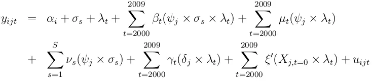
The baseline model is as follows:
yijt =αj +λt+β(ψj×postt) +εijt (1.9)
where:
ψj = log
backlog judge
j,2009
postt =
(
1 if year>2005
0 if year62005
In equation 1.9,yis an outcome of firmioperating in judicial districtj at time
t and postt is a dummy equal to 1 after 2005 and 0 otherwise. The interaction term between ψj — which captures court congestion37 — andpostt is meant to
35E.g., single-plant firms, firms above 30 employees that are selected with probability one in the
survey, firms that do not change the location of their headquarters in the years under study.
36This is because the PIA survey does not provide information on loans taken by each firm.
When I instead use data from the PINTEC survey my main outcome variable is firm access to external funds used to finance technological investment.
37As discussed in section 1.3.2, here I use the cross-sectional variation in court congestion for
capture the treatment intensity of the reform. I add year fixed effects and judicial districts fixed effects to control for the two main effects of the interaction. Year fixed effects are meant to capture common aggregate shocks that each year hit all firms in the same way. Judicial district fixed effects control for characteristics of each judicial district that do not vary across time and might be correlated both with the congestion of their civil courts and the average performance of firms operating under their jurisdiction.
In a framework that combines firm-level data with district-level regressors, the adjustment of standard errors is a key issue when making statistical inference. This is because the error term might be composed by a location-year component along with the idiosyncratic individual component (meaning: εijt = ηjt +ηijt).
The judicial district fixed effects take out the average from ηjt, but its demeaned time variation might still be serially correlated. In order to correct the estimates for potential serial correlation within judicial districts, I use one of the solutions proposed by Bertrand et al. (2004) — to average the data before and after the reform and run equation 1.9 taking the dependent variables in first differences. I define the pre-reform years as the period 2003–2005 and the post-reform years as the period 2006–2009. These two periods are as comparable as possible in Brazil in terms of political and aggregate economic variables in Brazil.38 I therefore
estimate equation 1.9 as follows:
∆yijt=α+βψj +uijt (1.10)
When estimating equation 1.10 I cluster standard errors at judicial district level to take into account correlation across firms within the same district.39
Estimating in first differences is the analog of taking out judicial district fixed effects. In fact, equation 1.10 also takes out firm fixed effects, implying that it also controls for time unvarying unobservable characteristics, not just at the judicial district level but also at the firm level.40
for court congestion in the pre-reform period. In Table 1.18 I show that, when limiting the sample only to those judicial districts for which data is available from the pre-reform period (the states of Rondonia and Mato Grosso do Sul), I get very similar coefficients on the main outcome variables using the 2004 or the 2009 level of court congestion.
38The Lula’s government has been in power from 2003 to 2010. Brazilian GDP experienced
average growth of 3.3% a year between 2003 and 2005 and 3.7% a year between 2006 and 2009. Results are robust to different definition of the pre period (e.g. 2000-2005) or of the post period (e.g. 2006-2008)
39All results are robust to clustering at higher levels of aggregation with respect to the judicial
district (e.g. micro-regions, macro-regions, state). This is because there might be spatial correla-tion across judicial districts.
40The relevant variation is within-firm between before and after the reform, ruling out
Fixed effects do not take care of district-level omitted variables that might cor-relate with court congestion and that, at the same time, might explain why firms benefited in different ways from the introduction of the reform. In Table 1.5, I check for systematic differences across judicial districts that are below and above the median level of court congestion. The table shows the average value of a set of covariates in the pre-reform period: average monthly household income, pop-ulation, number of bank agencies, alphabetization rate of individuals above 10 years, number of manufacturing firms, agricultural share of GDP, and industry share of GDP.41 Judicial districts above and below the median of court
conges-tion are different in a number of dimensions and (surprisingly) similar in others. For example, I do not find statistically significant differences in terms of popula-tion, number of registered manufacturing firms, or number of bank agencies. In other words, there is no sign of initial selection of firms into districts with better court enforcement. Districts with more congested courts, however, seem to be on average richer (higher average household income per month), to have a more alphabetized adult population, and to have a local economy that relies more on industry than on agriculture. All of these are potential problems because a hetero-geneous effect of the reform attributed to the congestion of courts might actually be due, for example, to poorer districts catching up in terms of per capita income at the same time that the reform was implemented.
To address this concern, I add to equation 1.10 a set of initial conditions at the judicial district level (Xj,t=0): average household income per month (which is
strongly correlated both with alphabetization and industry share on GDP), popu-lation, and the number of bank agencies in each judicial district in the year 2000. Given that the number of controls I can insert in the model is limited, my estimates might still suffer from omitted variable bias. Thus, I propose an instrumental vari-able strategy in section 1.6.4. Finally, I add to the model a dummy identifying the existence of bankruptcy courts (δj) and sector fixed effects (σs) to control for
dif-ferent trends across firms operating in difdif-ferent industries42so that the final model
I estimate is:
∆yijst=α+βψj +γδj +ξ0Xj,t=0+σs+uijst (1.11)
only 1.2 % of them changed judicial district.
41All covariates are measured in the year 2000, the year of the last Census before the reform.
42In all regressions, I exclude firms operating in CNAE sector 23: the oil-processing industry.

![(WSNs)[ ].RFIDidentifiesanobject(forexample,avehicle)usingauniqueidentifier ],withauniqueidentityandtheabilitytosenseandcollectinformationfromthesurroundingenvironment,andshare ].Therefore,trafficcongestionhasbecomeafundamentalproblemandamajorchallengeformos](data:image/gif;base64,R0lGODlhAQABAIAAAP///wAAACH5BAEAAAAALAAAAAABAAEAAAICRAEAOw==)