Modeling of DCT Coefficients in the H.264 Video Encoder-Edición Única

Monterrey, Nuevo León a

INSTITUTO TECNOLÓGICO Y DE ESTUDIOS SUPERIORES DE MONTERREY

PRESENTE.-Por medio de la presente hago constar que soy autor y titular de la obra denominada"

, en los sucesivo LA OBRA, en virtud de lo cual autorizo a el Instituto Tecnológico y de Estudios Superiores de Monterrey (EL INSTITUTO) para que efectúe la divulgación, publicación, comunicación pública, distribución, distribución pública y reproducción, así como la digitalización de la misma, con fines académicos o propios al objeto de EL INSTITUTO, dentro del círculo de la comunidad del Tecnológico de Monterrey.

El Instituto se compromete a respetar en todo momento mi autoría y a otorgarme el crédito correspondiente en todas las actividades mencionadas anteriormente de la obra.

De la misma manera, manifiesto que el contenido académico, literario, la edición y en general cualquier parte de LA OBRA son de mi entera responsabilidad, por lo que deslindo a EL INSTITUTO por cualquier violación a los derechos de autor y/o propiedad intelectual y/o cualquier responsabilidad relacionada con la OBRA que cometa el suscrito frente a terceros.

Nombre y Firma AUTOR (A)

Modeling of DCT Coefficients in the H.264 Video

Encoder-Edición Única

Title Modeling of DCT Coefficients in the H.264 Video Encoder-Edición Única

Authors Roberto Rivera Jiménez

Affiliation Campus Monterrey

Issue Date 2008-04-01

Item type Tesis

Rights Open Access

Downloaded 19-Jan-2017 06:44:23

INSTITUTO TECNOLÓGICO Y DE ESTUDIOS

SUPERIORES DE MONTERREY

CAMPUS MONTERREY

PROGRAMA DE GRADUADOS EN MECATRÓNICA Y TECNOLOGÍAS DE INFORMACIÓN

MODELING OF DCT COEFFICIENTS IN THE H.264 VIDEO ENCODER

THESIS

PRESENTED IN PARTIAL FULFILLMENT OF THE REQUIREMENTS FOR THE DEGREE OF:

MASTER IN TELECOMMUNICATIONS MANAGEMENT

BY:

ROBERTO RIVERA JIMÉNEZ

INSTITUTO TECNOLÓGICO Y DE ESTUDIOS

SUPERIORES DE MONTERREY

CAMPUS MONTERREY

PROGRAMA DE GRADUADOS EN MECATRÓNICA Y TECNOLOGÍAS DE INFORMACIÓN

The members of the Thesis Committee hereby recommend accepting the thesis presented by Roberto Rivera Jiménez in partial fulfillment of the requirements for the degree of

Master in Telecommunications Management

THESIS COMMITTEE:

____________________________________ Ramón Martín Rodríguez Dagnino, Ph.D. Thesis Advisor

____________________________________ José Ramón Rodríguez Cruz, Ph.D. Synodal

____________________________________ Roberto Rodríguez Said, Ph.D. Synodal

_________________________________________ Graciano Dieck Assad, Ph.D.

Director of the Graduate Program in Mechatronics and Information Technologies

MODELING OF DCT COEFFICIENTS IN THE H.264 VIDEO ENCODER

BY:

ROBERTO RIVERA JIMÉNEZ

THESIS

Presented to the Graduate Program in Mechatronics and Information Technologies

This work is a partial requirement for the degree of Master in Telecommunications Management

INSTITUTO TECNOLÓGICO Y DE ESTUDIOS SUPERIORES DE MONTERREY

Dedication

Acknowledgments

I would like to thank my parents, Roberto and Hilda, for their unconditional support and love; my brothers, Dante and Jesús, for all their help; and all my family for their motivation.

I would also like to thank my thesis advisor, Dr. Ramón Martín Rodríguez Dagnino, for his guidance and advice; and my thesis committee, Dr. José Ramón Rodríguez Cruz and Dr. Roberto Rodríguez Said, for their comments and observations that improved this work.

Thanks to the CONACYT for giving me the opportunity of realize my graduate studies.

Abstract

DCT stands for Discrete Cosine Transform (Ahmed, Natarajan, & Rao, 1974); it is an important tool used in video and image compression systems (Richardson, 2003). The understanding of the DCT coefficients’ statistical distribution has many applications; one of them is the rate control for video coding, which requires knowledge of the rate-distortion relation as a function of the encoder parameters and the video source statistics (Kamaci & Altunbasak, 2005)

Table of Contents

Dedication

... IV

Acknowledgments

... V

Abstract

... VI

Table of Contents

... VII

List of tables

... VIII

List of figures

... IX

Chapter I

OVERVIEW ... 1

I.1INTRODUCTION ... 1

I.2JUSTIFICATION ... 2

I.3OBJECTIVE ... 3

I.4ANTECEDENTS ... 3

I.5CONTRIBUTIONS ... 4

I.6STRUCTUREOFTHETHESIS... 4

Chapter II

DIGITAL VIDEO ... 5

II.1FUNDAMENTALS ... 5

II.1.1 Color formats ... 6

II.2COMPRESSION ... 7

II.2.1 Lossless compression ... 7

II.2.2 Lossy compression ... 8

II.2.3 Video Compression ... 8

II.2.4 Transmission Errors ... 9

II.3QUALITYMEASUREMENT ... 10

II.3.1 Subjective Quality Measurement ... 10

II.3.2 Objective Quality Measurement ... 10

Chapter III

VIDEO CODEC ... 12

III.1TEMPORALMODEL ... 13

III.1.1 Prediction from the Previous Video Frame ... 14

III.2SPATIALMODEL ... 14

III.2.1 Transformation ... 14

III.2.2 Quantization ... 16

III.3ENTROPYCODING ... 18

III.3.2 Run-Length Encodings ... 20

III.4DECODER ... 20

Chapter IV

THE H.264 ENCODER (VCL) ... 21

IV.1MACROBLOCKS ... 21

IV.2SLICESANDSLICEGROUPS... 22

IV.3MOTIONESTIMATION... 23

IV.4TRANSFORMATIONANDQUANTIZATION ... 24

IV.4.1 Transformation ... 24

IV.4.2 Quantization ... 26

IV.5ENTROPYCODING ... 27

IV.5.1 CAVLC ... 27

IV.5.2 CABAC ... 27

Chapter V

DCT MODELING ... 29

V.1LAPLACEPROBABILITYDENSITYFUNCTION ... 29

V.2GENERALIZEDGAUSSIANPROBABILITYDENSITYFUNCTION ... 30

V.2.1 Parameter Estimation ... 31

V.3CAUCHYPROBABILITYDENSITYFUNCTION ... 33

V.3.1 Parameter Estimation ... 34

Chapter VI

EXPERIMENTS ... 36

VI.1TESTENVIRONMENT ... 36

VI.1.1 Test sequences ... 37

VI.1.2 Generalized Gaussian... 42

VI.1.3 Cauchy ... 44

VI.2THE TEST ... 50

VI.2.1 Experimental Results ... 51

VI.3ENTROPYMODELSOFQUANTIZEDSOURCES ... 55

VI.3.1 Laplace ... 55

VI.3.2 Cauchy ... 56

VI.3.3 Generalized Gaussian... 56

VI.3.4 Experimental Results ... 57

VI.4DISTORTIONMODELSOFQUANTIZEDSOURCES ... 63

VI.4.1 Laplace ... 64

VI.4.2 Cauchy ... 64

VI.4.3 Generalized Gaussian... 65

VI.4.4 Experimental Results ... 65

VI.5CONCLUSIONSANDFURTHERWORK ... 73

Chapter VII

APPENDIXES ... 76

VII.1GENERALIZEDGAUSSIANENTROPYMODEL ... 76

VII.2GENERALIZEDGAUSSIANDISTORTIONMODEL ... 78

Chapter VIII

REFERENCES ... 86

Table III-1: Optimum binary coding procedure, obtained from Huffman (1952). ... 19

Table IV-1:Inverse 8x8 transform basis, obtained from (Bossen, 2002) ... 25

Table VI-1: Mean (GOP: IIIIIII) ... 38

Table VI-2: Mean (GOP: IBBPBBP_12) ... 38

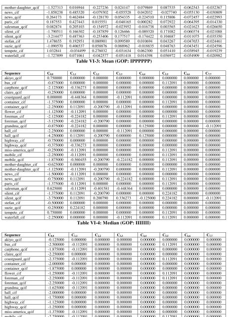
Table VI-3: Mean (GOP: IPPPPPP) ... 39

Table VI-4: Median (GOP: IIIIIII) ... 39

Table VI-5: Median (GOP: IBBPBBP_12) ... 40

Table VI-6: Median (GOP: IPPPPPP) ... 40

Table VI-7: Standard Deviation (GOP: IIIIIII) ... 41

Table VI-8: Standard Deviation (GOP: IBBPBBP_12) ... 41

Table VI-9: Standard Deviation (GOP: IPPPPPP) ... 42

Table VI-10: p Parameter (GOP: IIIIIII) ... 43

Table VI-11: p Parameter (GOP: IBBPBBP_12) ... 43

Table VI-12: p Parameter (GOP: IPPPPPP) ... 44

Table VI-13: Scale Parameter (GOP: IIIIIII) ... 44

Table VI-14: Scale Parameter (GOP: IBBPBBP_12) ... 45

Table VI-15: Scale Parameter (GOP: IPPPPPP) ... 45

Table VI-16: Chi2 results IIIIIII ... 52

Table VI-17: Chi2 results IBBPBBP_12 ... 53

Table VI-18: Chi2 results IPPPPPP ... 54

List of figures

Fig. II-1: Spatial and temporal sampling of a video sequence, obtained from Richardson (2003). ... 5

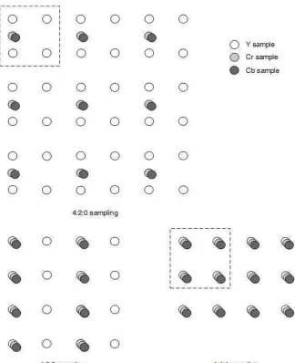
Fig. II-2: YCbCr sampling patterns, obtained from Richardson (2003). ... 7

Fig. II-3: Typical compression artifacts, obtained from Winkler, 2005 ... 9

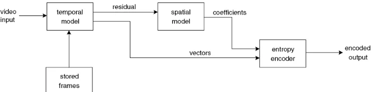
Fig. III-1: Video encoder block diagram, obtained from Richardson (2003). ... 13

Fig. III-2: Uniform Quantizer, obtained from Gray & Neuhoff (1998). ... 17

Fig. III-3: Quantization characteristics, obtained from Ghanbari (2003). ... 17

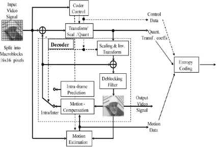
Fig. IV-1: Structure of H.264/AVC video encoder, obtained from Wiegand et al (2003). .. 21

Fig. IV-2: Basic coding structure for H.264/AVC for a macroblock, obtained from Wiegand et al. (2003). ... 23

Fig. IV-3: Fast implementation of the H.264 direct transform (top) and inverse transform (bottom), obtained from Malvar et al. (2003) ... 25

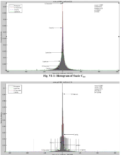
Fig. VI-1: Histogram of Suzie C0,0 ... 46

Fig. VI-2: Histogram of Akiyo C0,0 ... 46

Fig. VI-3: Histogram of Foreman C1,1 ... 47

Fig. VI-4: : Histogram of Carphone C3,3 ... 47

Fig. VI-5: Histogram of Flower C4,4 ... 48

Fig. VI-7: Histogram of Mobile C7,7 ... 49

Fig. VI-8: Histogram of Waterfall C7,7 ... 49

Fig. VI-9: Entropy of akiyo_qcif ... 57

Fig. VI-10: Entropy of bus_cif ... 57

Fig. VI-11: Entropy of carphone_qcif ... 58

Fig. VI-12: Entropy of claire_qcif ... 58

Fig. VI-13: Entropy of coastguard_qcif ... 58

Fig. VI-14: Entropy of container_cif ... 58

Fig. VI-15: Entropy of container_qcif ... 58

Fig. VI-16: Entropy of flower_cif ... 59

Fig. VI-17: Entropy of foreman_cif ... 59

Fig. VI-18: Entropy of foreman_qcif ... 59

Fig. VI-19: Entropy of grandma_qcif ... 59

Fig. VI-20: Entropy of hall_cif ... 59

Fig. VI-21: Entropy of hall_qcif ... 60

Fig. VI-22: Entropy of highway_cif ... 60

Fig. VI-23: Entropy of highway_qcif ... 60

Fig. VI-24: Entropy of miss-america_qcif ... 60

Fig. VI-25: Entropy of mobile_cif ... 60

Fig. VI-26: Entropy of mobile_qcif ... 61

Fig. VI-27: Entropy of mother-daughter_cif ... 61

Fig. VI-28: Entropy of mother-daughter_qcif ... 61

Fig. VI-29: Entropy of news_cif ... 61

Fig. VI-30: Entropy of news_qcif ... 61

Fig. VI-31: Entropy of paris_cif ... 62

Fig. VI-32: Entropy of salesman_qcif ... 62

Fig. VI-33: Entropy of silent_cif ... 62

Fig. VI-34: Entropy of silent_qcif ... 62

Fig. VI-35: Entropy of stefan_cif ... 62

Fig. VI-36: Entropy of suzie_qcif ... 63

Fig. VI-37: Entropy of tempete_cif ... 63

Fig. VI-38: Entropy of waterfall_cif ... 63

Fig. VI-39: Distortion of akiyo_qcif ... 66

Fig. VI-40: Distortion of bus_cif ... 66

Fig. VI-41: Distortion of carphone_qcif ... 66

Fig. VI-42: Distortion of claire_qcif ... 66

Fig. VI-43: Distortion of coastguard_qcif ... 67

Fig. VI-44: Distortion of container_cif ... 67

Fig. VI-45: Distortion of container_qcif ... 67

Fig. VI-46: Distortion of flower_cif ... 67

Fig. VI-47: Distortion of foreman_cif ... 68

Fig. VI-48: Distortion of foreman_qcif ... 68

Fig. VI-49: Distortion of grandma_qcif ... 68

Fig. VI-50: Distortion of hall_cif ... 68

Fig. VI-51: Distortion of hall_qcif ... 69

Fig. VI-53: Distortion of highway_qcif ... 69

Fig. VI-54: Distortion of miss-america_qcif ... 69

Fig. VI-55: Distortion of mobile_cif ... 70

Fig. VI-56: Distortion of mobile_qcif ... 70

Fig. VI-57: Distortion of mother-daughter_cif ... 70

Fig. VI-58: Distortion of mother-daughter_qcif ... 70

Fig. VI-59: Distortion of news_cif ... 71

Fig. VI-60: Distortion of news_qcif ... 71

Fig. VI-61: Distortion of paris_cif ... 71

Fig. VI-62: Distortion of salesman_qcif ... 71

Fig. VI-63: Distortion of silent_cif ... 72

Fig. VI-64: Distortion of silent_qcif ... 72

Fig. VI-65: Distortion of stefan_cif ... 72

Fig. VI-66: Distortion of suzie_qcif ... 72

Fig. VI-67: Distortion of tempete_cif ... 73

1

Chapter I

OVERVIEW

I.1 INTRODUCTION

The advances in video coding technology and standardization, together with the improvements in network infrastructures, storage capacity, and computing power are enabling an increasing number of video applications. Among these are: multimedia messaging, video conferencing, Internet video streaming, high-definition TV broadcasting, DVD, Blu-ray Disc, and HD DVD (Schwarz, Marpe, & Wiegand, 2007).

Video sources are by nature analog and they need to be digitally encoded before they can be stored in digital media or transmitted over digital telecommunications networks. The difficulty is the extensive amount of data required to represent them (Sharifi, 1995).

H.264/AVC (Advanced Video Coding) is a video codec standard of the International Telecommunication Union - Telecommunication Standardization Sector proposed in 2003 (ITU-T Rec. H.264, 2005). It is the result of the Joint Video Team (JVT) formed by the Moving Picture Experts Group (MPEG) and the ITU’s Video Coding Experts Group (Wenger, 2003). It is also known as MPEG-4 part 10 AVC (Wiegand, Sullivan, Bjøtegaard, & Luthra, 2003).

2

In H.264/AVC the only part standardized is the central decoder, this is achieved by restricting the encoded bitstream and syntax, and defining the decoding process of the syntax elements in such way that every standardized decoder will produce similar results when given an encoded bitstream that conforms to the constraints of the standard (Wiegand, Sullivan, Bjøtegaard, & Luthra, 2003). This allows maximal freedom to improve the implementations in a tailored way to specific applications (Wiegand et al., 2003).

Fig. I-1: Scope of video coding standardization, obtained from Wiegand et al. (2003)

I.2 JUSTIFICATION

DCT stands for Discrete Cosine Transform (Ahmed, Natarajan, & Rao, 1974) and it is an important tool used in video and image compression systems (Richardson, 2003). The understanding of the statistical distribution of the DCT coefficients can be useful in quantizer design and noise mitigation for image enhancement (Lam & Goodman, 2000). Entropy coding benefits from modeling the amplitude distribution of the DCT coefficients, and then using a collection of entropic codebooks each fitting a modeled PDF of the true data (Aiazzi, Alparone, & Baronti, 1999).

Knowledge of the DCT coefficients’ probability distribution is particularly important in rate control for video coding, “since the problems of bit allocation and quantization scale selection require knowledge of the rate-distortion relation as a function of the encoder parameters and the video source statistics” (Kamaci & Altunbasak, 2005).

3

I.3 OBJECTIVE

The objective of this thesis is to compare three theoretical Probability Density Functions (the Laplace, Cauchy and Generalized Gaussian) in terms of: how well they represent the empirical DCT coefficient data; how well the models based on them can predict the actual rate of the coded video; and how well the models based on them can predict the actual distortion of the coded video.

I.4 ANTECEDENTS

This section briefly describes some of the prior works in the subject of DCT coefficient modeling.

Reiningek & Gibson (1983) used the Laplacian, Gaussian and Gamma modeling in images and compared them using the Kolmogorov-Smirnov (KS) test of goodness-of-fit. They concluded that, for a large class of images, the DC coefficient was best modeled by a Gaussian PDF, and the AC coefficients were best modeled by a Laplacian distribution.

Müller (1993) used the Laplacian and Generalized Gaussian DCT modeling in images and compared them using the test of goodness-of-fit. His results showed that the shape parameter of the G.G. was generally far from the Laplacian case and the values were considerable lower in the G.G. case (thus it had a better fit than the Laplacian).

Birney & Fischer (1995) used the Laplacian and Generalized Gaussian DCT modeling in images, and designed quantizers and codes based on them. Their results showed that the ones based on the Generalized Gaussian PDF were always superior in Mean-squared Error than the ones based on Laplacian PDF, but by a little margin that did not outweigh the computational cost. Joshi & Fischer (1995), without doing the quantizer and code design, found similar results.

Lam & Goodman (2000) presented a rigorous mathematical analysis using a doubly stochastic model of images and used it to explain why previous observations from the literature lead to the proposal of the Laplacian and Gaussian PDF as a way to model the DCT coefficients.

4

differences between the predicted and the actual values) can be positive or negative.

Altunbasak & Kamaci (2004) proposed the use of the Cauchy PDF as a way to model the DCT coefficients in H.264. Their results showed that it performed better than the widely used Laplacian PDF. They also proposed exact analytical models for the Entropy and Distortion based on it. Kamaci, Altunbasak, & Mersereau (2005) expanded their previous results and proposed a Frame bit allocation scheme using the Cauchy PDF.

Syu (2005) showed exact analytical models for the Entropy and Distortion of the H.264 encoded video based on the Laplace PDF. Those had a very low computational cost and were specifically used in a resource limited encoder.

Sun et al. (2005) used the Generalized Gaussian Distribution in order to model the DCT coefficients in MPEG-4 encoded videos. They also proposed approximate analytical models for the Entropy and Distortion based on the Generalized Gaussian PDF.

I.5 CONTRIBUTIONS

Some of the contributions of this thesis are the comparisions of the Cauchy and the Generalized Gaussian Probability Density Functions; in the antecedents sections there is literature that compares each to the Laplace PDF, but a direct comparission between the two could not be found.

The main contribution of this work is the derivation of exact anaytical models for the Entropy and Distortion, based on the Generalized Gaussian PDF.

I.6 STRUCTURE OF THE THESIS

5

Chapter II

DIGITAL VIDEO

II.1 FUNDAMENTALS

A pixel, also called picture element or pel, is a digital sample of the intensity (of the color or the brightness) value of a picture at a single point (Symes, 2004).

Fig. II-1: Spatial and temporal sampling of a video sequence, obtained from Richardson (2003).

6

“The human eye contains more than 100 million sensors with a brightness control system that allows clear vision over a brightness range of more than ten million to one. The two eyes together with the brain give the ability to recognize objects in three-dimensional space” (Luther, 1997).

“The sensitivity of the human eye varies from color to color and from person to person, for the same color. In addition, two different persons may perceive the same color with the same intensity differently. Furthermore, the human eye is more sensitive to yellow or yellow-green than red and violet” (Ramírez-Velarde, 2004).

II.1.1 Color formats

An analog video camera produces three distinct continuous signals, one for each color component Red, Green and Blue; these three colors, are called the additive primaries. RGB is the standard for video cameras (Ramírez-Velarde, 2004).

Video coding often uses a color representation that has three components: , , and . Component is called luma and represents brightness. The two chroma components and represent the deviation from gray to blue and red, respectively (Sullivan & Wiegand, 2005).

7

Fig. II-2: YCbCr sampling patterns, obtained from Richardson (2003).

4:4:4 sampling means that the three components have the same resolution. The numbers indicate the relative sampling rate of each component in the horizontal direction. In 4:2:2 and have the same vertical resolution as but half the horizontal resolution. In 4:2:0 and each have half the horizontal and vertical resolution of . The term 4:2:0 is misleading because the numbers do not have a logical interpretation (Richardson, 2003). Because the human visual system is more sensitive to luma than chroma, the 4:2:0 sampling structure is the most widely used (Sullivan & Wiegand, 2005).

II.2 COMPRESSION

“Data compression can be viewed as a means for efficient representation of a digital source of data such as text, image, sound or any combination of all these types such as video. The goal of data compression is to represent a source in digital form with as few bits as possible while meeting the minimum requirement of reconstruction of the original” (Pu, 2006).

II.2.1 Lossless compression

8

Lossless compression works by taking away redundant data: “information that, if removed, can be recreated from the remaining data” (Symes, 2004).

II.2.2 Lossy compression

A compression method is lossy if it is not possible to reconstruct the original exactly from the compressed version. Lossy compression is also called irreversible compression (Pu, 2006).

Ideally, lossy compression removes irrelevant information, that would mean that the recipient cannot perceive that it is missing. Information that is close to irrelevant, would mean that the quality loss is small compared to the reduction in the size of data (Symes, 2004).

“Approximate reconstruction may be desirable since it may lead to more effective compression. However, it often requires a good balance between the visual quality and the computation complexity” (Pu, 2006).

“Data such as multimedia images, video and audio are more easily compressed by lossy compression techniques because of the way that human visual and hearing systems work” (Pu, 2006). Lossy video compression systems are based on the principle of removing subjective redundancy, data that can be removed without radically affecting the viewer’s quality perception (Richardson, 2003).

II.2.3 Video Compression

Video compression is the process of compacting or condensing a digital video sequence into a smaller number of bits (Richardson, 2003).

Compression involves a complementary pair of systems, a compressor (encoder) and a decompressor (decoder). The encoder converts the source data into a compressed form prior to transmission or storage and the decoder converts the compressed form back into a representation of the original video data. “The encoder/decoder pair is often described as a CODEC (enCOder/ DECoder)” (Richardson, 2003).

According to Yuen & Wu (as cited in Winkler, 2005), a variety of artifacts can be distinguished in a compressed video sequence:

9

• Blur manifests itself as a loss of spatial detail and a reduction of edge sharpness.

• Color bleeding is the smearing of colors between areas of strongly differing chrominance.

• Slanted lines often exhibit the staircase effect

• Ringing is fundamentally is most evident along high-contrast edges in otherwise smooth areas.

• False edges. • Jagged motion.

• Mosquito noise, a temporal artifact seen mainly in smoothly textured regions as luminance/chrominance fluctuations around high-contrast edges or moving objects.

• Flickering appears when a scene has high texture content.

• Aliasing can be noticed when the content of the scene is above the Nyquist rate, either spatially or temporally.

Fig. II-3: Typical compression artifacts, obtained from Winkler, 2005

II.2.4 Transmission Errors

10

application, both have the same effect: part of the media stream is not available (Winkler, 2005).

Such losses can affect both the semantics and the syntax of the media stream. When the losses affect syntactic information, not only the data relevant to the lost block are corrupted, but also any other data that depend on this syntactic information. (Winkler, 2005).

II.3 QUALITY MEASUREMENT

II.3.1 Subjective Quality Measurement

Subjective evaluation that directly reflects human perception is considered to be the most accurate method of video quality measurement. It requires a large number of evaluators and a specially designed testing room (Choe & Lee, 2007).

Subjective testing for visual quality assessment has been formalized in ITU-R Rec. BT.500-11 (2002; as referenced in Winkler, 2005) and ITU-T Rec. P.910 (1999; as referenced in Winkler, 2005), which suggest “standard viewing conditions, criteria for the selection of observers and test material, assessment procedures, and data analysis methods” (Winkler, 2005).

“The perception of visual quality is influenced by spatial fidelity (how clearly parts of the scene can be seen) and temporal fidelity (whether motion appears natural and ‘smooth’). Other important influences on perceived quality include visual attention (an observer perceives a scene by fixating on a sequence of points in the image rather than by taking in everything simultaneously) and the so-called ‘recency effect’ (our opinion of a visual sequence is more heavily influenced by recently-viewed material than older video material). All of these factors make it very difficult to measure visual quality accurately and quantitatively” (Richardson, 2003).

Another disadvantage is that subjective quality measurement cannot be applied in real time, that is, during the encoding process (Choe & Lee, 2007).

II.3.2 Objective Quality Measurement

11

For a transform of size , the II.3.2.1 Mean Squared Error (MSE) is defined as:

1 !

"# !

"#

Where is the actual value, and is the reference or reconstructed value as (Richardson, 2003).

For a transform of size , the II.3.2.1 Mean Absolute Error (MAE) is defined as:

$ 1 % %

!

"# !

"#

Where is the actual value, and is the reference or reconstructed value as (Richardson, 2003).

For a transform of size , the II.3.2.1 Sum of Absolute Errors (SAE) is defined as:

$ % %

!

"# !

"#

Where is the actual value, and is the reference or reconstructed value as (Richardson, 2003).

The Peak Signal to Noise Ratio (PSNR) depends on the MSE between an original and a reconstructed image or video frame, “relative to 2' 1 (the square of the highest-possible signal value in the image, where ( is the number of bits per image sample)”. (Richardson, 2003).

) * 10,-. 2

' ₁

12

Chapter III

VIDEO CODEC

A video CODEC encodes a source image or video sequence into a compressed form and decodes it to produce a copy or approximation of the source sequence (Richardson, 2003).

“The basic communication problem may be posed as conveying source data with the highest fidelity possible within an available bit rate, or it may be posed as conveying the source data using the lowest bit rate possible while maintaining specified reproduction fidelity. In either case, a fundamental tradeoff is made between bit rate and fidelity. The ability of a source coding system to make this tradeoff well is called its coding efficiency or rate-distortion performance, and the coding system itself is referred to as a codec” (Sullivan & Wiegand, 2005).

According to Sullivan & Wiegand (2005), video codecs are primarily characterized in terms of:

• Throughput of the channel: a characteristic influenced by the transmission channel bit rate and the amount of protocol and error-correction coding overhead incurred by the transmission system. • Distortion of the decoded video: distortion is primarily induced by the

13

• Delay (startup latency and end-to-end delay): Delay characteristics are influenced by many parameters, including processing delay, buffering, structural delays of video and channel codecs, and the speed at which data are conveyed through the transmission channel. • Complexity (in terms of computation, memory capacity, and memory access requirements). The complexity of the video codec, protocol stacks, and network. Hence, the practical source coding design problem is posed as follows: given a maximum allowed delay and a maximum allowed complexity, achieve an optimal tradeoff between bit rate and distortion for the range of network environments envisioned in the scope of the applications. The various application scenarios of video communication show very different optimum working points, and these working points have shifted over time as the constraints on complexity have been eased by Moore’s law and as higher bit-rate channels have become available.

Fig. III-1: Video encoder block diagram, obtained from Richardson (2003).

A video encoder consists of three main functional units: a temporal model, a spatial model and an entropy coder (Richardson, 2003).

III.1 TEMPORAL MODEL

14

The input to the temporal model is an uncompressed video sequence. “The output of the temporal model is a residual frame (created by subtracting the prediction from the actual current frame) and a set of model parameters, typically a set of motion vectors describing how the motion was compensated” (Richardson, 2003).

III.1.1 Prediction from the Previous Video Frame

The simplest method of temporal prediction is to use the previous frame as the predictor for the current frame. “The obvious problem with this simple prediction is that a lot of energy remains in the residual frame and this means that there is still a significant amount of information to compress after temporal prediction. Much of the residual energy is due to object movements between the two frames and a better prediction may be formed by compensating for motion between the two frames” (Richardson, 2003).

“Changes between video frames may be caused by object motion, camera motion, uncovered regions and lighting changes. With the exception of uncovered regions and lighting changes, these differences correspond to pixel movements between frames. It is possible to estimate the trajectory of each pixel between successive video frames, producing a field of pixel trajectories” (Richardson, 2003).

III.2 SPATIAL MODEL

The residual frame forms the input to the spatial model which makes use of similarities between neighboring samples in the residual frame to reduce spatial redundancy. Usually this is achieved by applying a transform to the residual samples and quantizing the results. The output of the spatial model is a set of quantized transform coefficients (Richardson, 2003).

III.2.1 Transformation

“A transform is a mathematical rule that may be used to convert one set of values to a different set” (Symes, 2004).

15

III.2.1.1 DCT

Ahmed, Natarajan & Rao (1974) defined the DCT of a data sequence X(m), m = 0, 1, …, (M - 1) as:

∑

X X m

M G

∑

G k=1, 2, …, (M-1)

Where Gx(k) is the kth DCT coefficient.

The inverse cosine discrete transform (IDCT) is defined as:

∑

X m=0, 1, …, (M-1)

If the inverse transform is written in matrix form and Λis the (M × M) matrix that denotes the cosine transformation, then the orthogonal property can be expressed as:

] [ 2 I

M

TΛ=

Λ

where ΛT _{is the transpose of Λ and [}

I ] is the (M × M) identity matrix (Ahmed et al. 1974).

“The performance of the DCT, particularly important in transform coding, is associated with the Karhunen-Loève transform. KLT is an optimal transform for data compression in a statistical sense because it decorrelates a signal in the transform domain, packs the most information in a few coefficients, and minimizes mean-square error between the reconstructed and original signal compared to any other transform. However, KLT is constructed from the eigenvalues and the corresponding eigenvectors of a covariance matrix of the data to be transformed; it is signal-dependent, and there is no general algorithm for its fast computation” (Britanak, 2001).

16

/ 0 1: 3 5_{4!6'7 82 9:':7cos}>( _{? , (, 0,1, … ,}

/ 0 11: 3 55₆

'7 82 B:7cos> 2( 1₂ C , (, 0,1, … , 1

/ 0 111: 3 555_{6'7 82 B:'cos}> 2 1 (

2 C , (, 0,1, … , 1

/ 0 1D: 3 5E₆

'7 82 Bcos > 2( 1 2₄ 1 C , (, 0,1, … , 1

:G H

1

√2 J 0 -K J

1 -LMNKOPQN R

Where is assumed to be an integer power of 2 (Wang & Hunt, 1985; as cited in Britanak 2001).

III.2.2 Quantization

The quantizer can be defined as consisting of a set of intervals or cells

S ; P U VW, where the index set V is ordinarily a collection of consecutive integers beginning with 0 or 1, together with a set of reproduction values or points or levels

SX ; P U VW, so that the overall quantizer Y is defined by Y Z X for Z U , which can be expressed concisely as (Gray & Neuhoff, 1998):

Y Z X 1_[\ Z

Where the indicator function 1_[ Z is 1 if Z U and 0 otherwise. Assuming that is a partition of the real line. That is, the cells are disjoint and exhaustive (Gray & Neuhoff, 1998).

17

allowed, then all but two cells will have width Δ and the outermost cells will be semi-infinite” (Gray & Neuhoff, 1998).

Fig. III-2: Uniform Quantizer, obtained from Gray & Neuhoff (1998).

The class of quantizer that has been used in all standard video codecs is based around the uniform threshold quantizer (UTQ). It has equal step sizes with reconstruction values nailed to the centroid of the steps. (Ghanbari, 2003)

Fig. III-3: Quantization characteristics, obtained from Ghanbari (2003).

The two key parameters that define a UTQ are the threshold value, th, and the step size, q. “The centroid value is typically defined mid way between quantization intervals. Note that, although AC transform coefficients have non-uniform characteristics, and hence can be better quantized with non-uniform quantizer step sizes (the DC coefficient has a fairly uniform distribution), bit rate control would be easier if they were quantized linearly. Hence, a key property of UTQ is that the step sizes can be easily adapted to facilitate rate control”. (Ghanbari, 2003).

In practice, rather than transmitting a quantized coefficient to the decoder, its ratio to the quantizer step size, called the quantization index, I.

1 _, ` a _, `_{Y b}

At the decoder, the reconstructed coefficients, c _, ` , after inverse quantization are given by:

c _{_, ` d1 _, ` e}1

18

One of the main problems of linear quantizers in DPCM is that for lower bit rates the number of quantization levels is limited and hence the quantizer step size is large. In coding of plain areas of the picture, if a quantizer with an even number of levels is used, then the reconstructed pixels oscillate between -q/2 and q/2. This type of noise at these areas, in particular at low luminance levels, is visible and is called granular noise. (Ghanbari, 2003).

Larger quantizer step sizes with an odd number of levels (dead zone) reduce the granular noise, but cause loss of pixel resolution at the plain areas. This type of noise when the quantizer step size is relatively large is annoying and is called contouring noise. (Ghanbari, 2003).

III.3 ENTROPY CODING

Entropy Coding is a process by which discrete-valued source symbols are represented in a manner that takes advantage of the relative probabilities of the various possible values of each source symbol (Sullivan & Wiegand, 2005).

The parameters of the temporal model and the spatial model are compressed by the entropy encoder. This removes statistical redundancy in the data and produces a compressed bit stream or file. “A compressed sequence consists of coded motion vector parameters, coded residual coefficients and header information” (Richardson, 2003).

The entropy of an information source is defined as (Shannon, 1948):

g J ,-._J1

'

"!

J ,-.J

'

"!

for independent symbols. Where J is the probability of symbol h and ( is the number of symbols.

If the logarithm of the base 2 is used, the entropy is represented in terms of bits, which is a contraction of binary unit (Abramson, 1963).

Without entropy coding, a quantizer with i levels would require ,-. 3i6 bits to represent each sample at the quantizer output. Entropy coding reduces this value to g j k ,-. 3i6 (Sharifi, 1995).

19

III.3.1 Huffman Coding

Huffman (1952) proposed a technique for the construction of minimum-redundancy codes. A “minimum-minimum-redundancy code” is defined as an ensemble code which, for a message ensemble consisting of a finite number of members, N, and for a given number of coding digits, D, yields the lowest possible average message length (Huffman, 1952).

ilm ) P i P

Where is the number of messages in the ensemble, ) P is the probability of the Pth message and i P is the number of coding digits assigned to it (Huffman, 1952).

The procedure involves two processes, source reduction followed by codeword construction. In the source reduction, the two least probable symbols are combined, leaving an alphabet with one less symbol. The combined symbol has a probability equal to the sum of the probabilities of the two original symbols. The process is repeated until there are only two symbols. The codeword construction begins allocating the codes 0 and 1 to the two remaining symbols. Conventionally 0 is used to represent the higher priority and 1 the lower priority. Then, each composite symbol is spited by appending 0 and 1 to its code, and the process continues until all the composite symbols have been reduced to original symbols of the alphabet (Symes, 2004).

20

III.3.2 Run-Length Encodings

Many compression methods are based on run-length encoding (RLE). Imagine a binary string. Let J be the probability that a zero appears and 1 J the probability that a one appear. If J is large, there will be runs of zeros, suggesting the use of RLE to compress the string. The probability of a run of ( zeros is J', and the probability of a run of ( zeros followed by a 1 is J' 1 J indicating that run lengths are distributed geometrically (Salomon, 2007).

Golomb (1966) proposed the following encoding procedure: Calculate:

n log 2_{log J}

That is Jq 1/2. The results will be most readily applicable for those J such that n is an integer (Golomb, 1966).

By computing:

Y s_nt( K ( Yn u vlog n w

The code is constructed in two parts; the first is the value of the quotient Y, coded in unary; the second is the binary value of the remainder K coded in a special way. The first 2x n values of K are coded, as unsigned integers, in

u 1 bits each, and the rest are coded in u bits each. The case where n is a power of 2 is special because it does not require u 1 bit codes. Once a Golomb code is decoded, the relation ( K Yn and the values of Y and K can be used to easily reconstruct ( (Salomon, 2007).

III.4 DECODER

21

Chapter IV

THE H.264 ENCODER (VCL)

Fig. IV-1: Structure of H.264/AVC video encoder, obtained from Wiegand et al (2003).

According to Wiegand et al. (2003), the H.264/AVC design covers a Video Coding Layer (VCL), which is designed to efficiently represent the video content, and a Network Abstraction Layer (NAL), which formats the VCL representation of the video and provides header information in a manner appropriate for transference by a variety of transport layers or storage media.

In this chapter the encoding function of the VCL is briefly explained. The NAL is out of the scope of this thesis.

IV.1 MACROBLOCKS

22

samples of each of the two chroma components. Macroblocks are the basic building blocks of the standard for which the decoding process is specified. (Wiegand, Sullivan, Bjøtegaard, & Luthra, 2003).

IV.2 SLICES AND SLICE GROUPS

“Slices are a sequence of macroblocks which are processed in the order of a raster scan when not using FMO (Flexible Macroblock Ordering). A picture may be split into one or several slices. A picture is therefore a collection of one or more slices in H.264/AVC. Slices are self-contained in the sense that given the active sequence and picture parameter sets, their syntax elements can be parsed from the bitstream and the values of the samples in the area of the picture that the slice represents can be correctly decoded without use of data from other slices provided that utilized reference pictures are identical at encoder and decoder” (Wiegand, Sullivan, Bjøtegaard, & Luthra, 2003).

According to Wiegand, et al. (2003), each slice can be coded using different coding types as follows:

• I slice: A slice in which all macroblocks of the slice are coded using intra prediction.

• P slice: In addition to the coding types of the I slice, some macroblocks of the P slice can also be coded using inter prediction with at most one motion-compensated prediction signal per prediction block.

• B slice: In addition to the coding types available in a P slice, some macroblocks of the B slice can also be coded using inter prediction with two motion-compensated prediction signals per prediction block. The above three coding types are very similar to those in previous standards with the exception of the use of reference pictures as described below. The following two coding types for slices are new. • SP slice: A so-called switching P slice that is coded such that efficient switching between different pre-coded pictures becomes possible.

• SI slice: A so-called switching I slice that allows an exact match of a macroblock in an SP slice for random access and error recovery purposes.

23

even when they are predicted using different reference frames. Due to this property, SP-frames can be used instead of I-frames in such applications as bitstream switching, splicing, random access, fast forward, fast backward, and error resilience/recovery. At the same time, since SP-frames unlike I-frames are utilizing motion-compensated predictive coding, they require significantly fewer bits than I-frames to achieve similar quality. In some of the mentioned applications, SI-frames are used in conjunction with SP-SI-frames. An SI-frame uses only spatial prediction as an I-frame and still reconstructs identically the corresponding SP-frame, which uses motion-compensated prediction. (Karczewicz & Kurceren, 2003).

Fig. IV-2: Basic coding structure for H.264/AVC for a macroblock, obtained from Wiegand et al. (2003).

IV.3 MOTION ESTIMATION

24

IV.4 TRANSFORMATION AND QUANTIZATION

IV.4.1 Transformation

Similar to previous video coding standards, H.264/AVC utilizes transform coding of the prediction residual. Instead of discrete cosine transform (DCT), a separable integer transform with similar properties as DCT is used. This characteristic of the transform in H.264 makes it different than the previous video codecs (Wiegand, Sullivan, Bjøtegaard, & Luthra, 2003).

For the DCT of the luma components the H.264 can use a 4x4 or a 8x8 DCT transform (Schwarz, Marpe, & Wiegand, 2007).

Malvar, Hallapuro, Karczewicz (2002, as cited in Malvar et al. 2003) proposed the following 4x4 transformation for H.264:

The integer transform used in H.264 is obtained by rounding the scaled entries of the DCT matrix to nearest integers:

H = round { α _{ADCT }}

Where ADCT is the DCT matrix. Setting α _{= 0.25 leads to the new} set of coefficients {a=1, b=2, c=1}

H =             − − − − − − 1 2 2 1 1 1 1 1 2 1 1 2 1 1 1 1

For the inverse transform, they proposed in H the scaling the oddsymmetric basis functions by ½; that is, replacing the rows [2 1 1 -2] and [1 -2 2 -1] by [1 1/2 -1/2 -1] and [1/2 -1 1 -1/-2], respectively. That way, the sum of absolute values of the odd functions is halved to three. The inverse transform matrix is then defined by:

25

Where the tilde indicates that inv is a scaled inverse of H.

“The multiplications by ½ can be implemented by sign-preserving 1-bit right shifts, so all decoders produce identical results. A key observation is that the small errors caused by the right shifts are compensated by the 2-bit gain in the dynamic range of the input to the inverse transform” (Malvar, Hallapuro, Karczewicz, & Kerofsky, 2003).

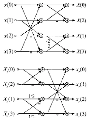
Fig. IV-3: Fast implementation of the H.264 direct transform (top) and inverse transform (bottom), obtained from Malvar et al. (2003)

In a similar way, Bossen (2002) proposed the 8x8 transform for H.264.

1 12/8 1 10/8 1 6/8 ½ 3/8

1 10/8 1/2 -3/8 -1 -12/8 -1 -6/8

1 6/8 -1/2 -12/8 -1 3/8 1 10/8

1 3/8 -1 -6/8 1 10/8 -1/2 -12/8

1 -3/8 -1 6/8 1 -10/8 -1/2 12/8

1 -6/8 -1/2 12/8 -1 -3/8 1 -10/8

1 -10/8 1/2 3/8 -1 12/8 -1 6/8

1 -12/8 1 -10/8 1 -6/8 ½ -3/8

Table IV-1:Inverse 8x8 transform basis, obtained from (Bossen, 2002)

Wien (2003) presents the concept of variable block size transform coding. The scheme is called adaptive block-size transforms (ABT), indicating the adaptation of the transform block size to the block size used for motion compensation.

26

other hand, larger transforms introduce more ringing artifacts caused by quantization than small transforms do. By choosing the transform size according to the signal properties, the tradeoff between energy compaction and preserved detail on the one hand and ringing artifacts on the other can be optimized. (Wien, 2003).

IV.4.2 Quantization

“In lossy compression, quantization is the step that introduces signal loss, for better compression” (Malvar, Hallapuro, Karczewicz, & Kerofsky, 2003). To avoid divisions, the H.264 implements new formulas for quantization:

{

}

) ,

(i j sign X i j X i j A Q f L

Xq = + L >>

) ( ) , ( ) ,

(i j X i j B Q

X_r = _q

N e X

H

x_r =( T _r +2N−1 )>>

Where, e = [1 1 1 1]T ; Q varies from zero to Qmax, and “the association of quantization parameters A(Q) and B(Q) are such that zero corresponds to the finest quantization and Qmax the coarsest quantization” (Malvar, Hallapuro, Karczewicz, & Kerofsky, 2003).

A quantization parameter is used for determining the quantization of transform coefficients in H.264/AVC. The parameter can take 52 values. These values are arranged so that an increase of 1 in quantization parameter means an increase of quantization step size by approximately 12% (an increase of 6 means an increase of quantization step size by exactly a factor of 2 (Wiegand, Sullivan, Bjøtegaard, & Luthra, 2003).

The code of the subroutine used to convert the quantization parameter QP, into the quantizer step size is the following (Sühring, 2007):

double QP2Qstep( int QP ) {

int i;

double Qstep;

static const double QP2QSTEP[6] = { 0.625, 0.6875, 0.8125, 0.875, 1.0, 1.125 }; Qstep = QP2QSTEP[QP % 6];

for( i=0; i<(QP/6); i++) Qstep *= 2;

27

IV.5 ENTROPY CODING

In H.264/MPEG4-AVC, many syntax elements are coded using the same highly-structured infinite-extent variable-length code (VLC), called a zero-order exponential-Golomb code. A few syntax elements are also coded using simple fixed-length code representations. For the remaining syntax elements, two types of entropy coding are supported, CAVLC and CABAC (Marpe, Wiegand, & Sullivan, 2006).

When using the first entropy-coding configuration, which is intended for lower-complexity implementations, the exponential-Golomb code is used for nearly all syntax elements except those of quantized transform coefficients (Marpe et al., 2006).

“The simpler entropy coding method uses a single infinite-extent codeword table for all syntax elements except the quantized transform coefficients. Thus, instead of designing a different VLC table for each syntax element, only the mapping to the single codeword table is customized according to the data statistics. The single codeword table chosen is an exp-Golomb code with very simple and regular decoding properties” (Wiegand et al. 2003)

IV.5.1 CAVLC

In the Context-adaptive variable length coding (CAVLC) entropy coding method, the number of nonzero quantized coefficients (N) and the actual size and position of the coefficients are coded separately. After zigzag scanning of transform coefficients, their statistical distribution typically shows large values for the low frequency part decreasing to small values later in the scan for the high-frequency part (Wiegand et al., 2003).

When using CAVLC, the encoder switches between different VLC tables for various syntax elements, depending on the values of the previously transmitted syntax elements in the same slice. Since the VLC tables are designed to match the conditional probabilities of the context, the entropy coding performance is improved from that of schemes that do not use context-based adaptivity (Marpe, Wiegand, & Sullivan, 2006).

IV.5.2 CABAC

28

nonbinary syntax elements to sequences of bits referred to as bin strings. The bins of a bin string can each be processed in either an arithmetic coding mode or a bypass mode. The latter is a simplified coding mode that is chosen for selected bins such as sign information or lesser-significance bins in order to speed up the overall decoding (and encoding) processes. The arithmetic coding mode provides the largest compression benefit, where a bin may be context-modeled and subsequently arithmetic encoded. (Marpe, Wiegand, & Sullivan, 2006).

29

Chapter V

DCT MODELING

V.1 LAPLACE PROBABILITY DENSITY FUNCTION

A random variable y is distributed as Laplacian, or double exponential, if its probability density function (PDF) is given by (Evans, Hastings, & Peacock, 1993):

i Z; z, { _{2| N}1 }~ •}, Z U €

Where z U €, { • 0, and | ‚ƒ„…!/ .

The C.D.F. is defined by (Evans, Hastings, & Peacock, 1993):

† Z ‡

1

2 N }• ~}, Z ˆ z 1 1_{2 N} }~ •}, Z ‰ z

30

V.2 GENERALIZED GAUSSIAN PROBABILITY DENSITY

FUNCTION

A random variable y is distributed as generalized Gaussian if its probability density function (pdf) is given by (Domínguez-Molina, González-Farías, & Rodríguez-Dagnino, 2001):

.. Z; z, {, J _{2Γ 1 1/J $ J, { N}1 Š ~ •‹ G,ƒ Š

Œ

, Z U €

Where z U €, J, { • 0, and $ J, { ‚ƒ„• !/G • Ž/G …

!/ .

Γ | is the Gamma function defined as (Abramowitz & Stegun, 1972):

Γ | • `‘ !<sub>N</sub> m<sub>•`</sub> #

The parameter z is the mean, the function $ J, { is a scaling factor which allows that D^K y { , and J is the shape parameter.

When J 1, the G.G. corresponds to a Laplacian distribution, J 2 corresponds to a Gaussian distribution, whereas in the limiting cases J ’ ∞ it converges to a uniform distribution in ”z √3{, z √3{–, and when J ’ 0 the distribution becomes a degenerate one in Z z (Domínguez-Molina, González-Farías, & Rodríguez-Dagnino, 2001).

Using the following property of the Gamma function:

Γ — 1 zΓ —

.. Z; z, {, J _{2Γ 1/J $ J, { N}J Š ~ •‹ G,ƒ Š

Œ

, Z U €

31

† Z

™ š š › š š

œ _{Γ •1J,•$ J, { ž}z Z Gž

2Γ Ÿ1J , Z k z

1 Γ •1J,• Z z $ J, { ž

G

ž

2Γ Ÿ1J , Z • z

R

Where Γ |, — is the upper incomplete gamma function, defined as (Abramowitz & Stegun, 1972):

Γ |, — • `‘ !<sub>N</sub> m<sub>•`</sub> ¡

V.2.1 Parameter Estimation

There are many methods to find the J parameter for the Generalized Gaussian PDF, most of them are either based on the maximum likelihood or on the the moments (Varanasi & Aazhang, 1989); there is also a method based on entropy matching (Aiazzi et al., 1999).

The Maximum Likelihood estimate of the J parameter is the root of the equation:

¢ Ÿ1J 1 log J

J J ,-. £1 1( |Z |G

'

"!

¥ ∑ |Z |'"!_{∑ |Z |'} G,-.|Z |_G

"! 0

Where:

¢ § ¨ • 1 L! © ! _{1 L} !_•L #

and ¨ 0.577 … denotes the Euler constant (Du, 1991; as cited in Müller, 1993; and in Joshi & Fisher, 1995).

The Entropy-Matching Method (Aiazzi, Alparone, & Baronti, 1999) uses the Entropy of the Generalized Gaussian source:

M-- _{J,( 2}1 log ® J

32

And the zero order entropy obtained after quantization:

g_# ) Pj ,-. 3) Pj 6

Where ) Pj is the probability that a coefficient is quantized to Pj, where

SP 0, e1, e2, … W and j is the quantizer step size.

Then, assuming that the standard deviation { ° j, the approximation:

g# ± M-- ,-. j

Can be used and then solve numerically for the parameter J (Aiazzi, Alparone, & Baronti, 1999).

The methods based on Moments consist of equating an appropriate number of sample moments to the corresponding parametric moments of the distribution (Varanasi & Aazhang, 1989).

In general, the (th moment of a random variable y is defined by (León-García, 1994):

3y'_{6 • Z}'_²

† Z •Z ‘

‘

One well-known method based on moments was first proposed by Mallat (1989) and was gradually improved in (Sharifi & León-García, 1995), (Rodríguez-Dagnino & León-García, 1998), (Domínguez-Molina, González-Farías, & Rodríguez-Dagnino, 2001). It can be resumed as follows:

Calculate:

J Γ Ÿ2J Γ Ÿ1J ΓŸJ 3

³ y |y|_y

33

|y| £1₍ |y z|

'

"!

¥

y 1₍ |y z|

'

"!

Then, by making

J ³ y

Solve numerically for J (Domínguez-Molina, González-Farías, & Rodríguez-Dagnino, 2001).

Summarizing, the Maximum Likelihood methods are among the most accurate for the estimation of the J parameter, nevertheless, their theoretical formulation and numerical solution make them unsuitable for real-time applications (Aiazzi, Alparone, & Baronti, 1999). The Entropy Matching method proposed in Aiazzi et al. (1999) depends on the assumption { ° j, which is restricted to small values of the quantizer step size. The methods based on the Moments, in general, are less accurate than the Maximum Likelihood methods; however they have the advantage of being more computationally efficient.

In this thesis, the method for the estimation of the J parameter explained in Domínguez-Molina et al. (2001) was used because of its relative effectiveness and efficiency; also because it has been successfully used in Sun et al. (2005).

V.3 CAUCHY PROBABILITY DENSITY FUNCTION

A random variable y is distributed as Cauchy if its probability density function (PDF) is given by:

u^_uMX Z; ^, | _| |/>_{Z ^ , Z U €}

Where ^ U € and | • 0. The parameter ^ is the location, and | is the scale (Koutrouvelis, 1982).

“The Cauchy distribution is unimodal and symmetric, with much heavier tails than the normal. The probability density function is symmetric about ^, with upper and lower quartiles, ^ e |” (Evans, Hastings, & Peacock, 1993).

34

† Z 1_{2 > tan}1 !ŸZ ^_|

V.3.1 Parameter Estimation

There are many methods to find the scale parameter for the Cauchy PDF, some are based in the maximum likelihood and others on order statistics. For a list of references see (Koutrouvelis, 1982).

The maximum likelihood estimators of ^ and | are the solutions of the equations:

1

( 1 3 Z 2 ^ /|6

'

"!

1

1

( 1 3 Z2Z ^ /|6

'

"!

^

Where ( is the sample size (Krishnamoorthy, 2006).

For the location parameter, “the maximum likelihood estimator is consistent and asymptotically efficient; unfortunately it is difficult to calculate and interpret. The sample median, although inefficient, is the simplest consistent estimator and would probably be used in practice” (Rothenberg, Fisher, & Tilanus, 1964).

Because the moments of the Cauchy PDF doesn’t exist (Krishnamoorthy, 2006), the methods based on moments can’t be applied to estimate the location or scale parameters.

Kamaci et al. (2005) propose a simple and computationally efficient estimation method for the scale parameter, which they used for their experiments on entropy and distortion. It can be resumed as follows:

Let ·_† Z be the empirical CDF obtained from the DCT histogram. They claim that this is the CDF of a Cauchy source with location parameter ^ 0 and scale parameter |.

·_{† Z ± † Z} 1

2 > tan1 !ŸZ|

35

† |Z| ) y k |Z| _{> tan}2 !ŸZ_|

And solving it for |

| Z

tan •>2 † |Z| ž

For some threshold Z. A proper selection of Z would be to set it equal to |, but because it’s not known, they experimentally found its range to be in the interval [0,3] and select Z 2 (Kamaci et al., 2005).

Although their method is computationally efficient, it is not very accurate. In order to improve it, a few modifications have been made here. First, the use of † Z instead of † |Z| , this comes at the cost of processing more elements of the DCT histogram.

·_{† Z ± † Z} 1

2 > tan1 !ŸZ|

And solving it for |

| _{tan >3} Z

† Z 1/26

The second modification is not selecting a fixed value of the threshold Z, instead, selecting the positions of the histogram that make

† Z 30.7, 0.8, 0.9, 0.9996, thus obtaining

|” † Z – 3| 0.7 , | 0.8 , | 0.9 , | 0.999 6.

It’s evident that the Cauchy PDF has its maximum when Z ^ 0, hence

max u^_uMX Z; ^, | |/>_{| >|}1

This can be used as a way to select |, which will be the element of |” _† Z – that satisfies | • 0 and minimizes:

Š)¼ _>|Š1

36

Chapter VI

EXPERIMENTS

VI.1 TEST ENVIRONMENT

The tests were performed using the JM encoder (Sühring, 2007) version 13.2, with the following parameters common to all tests:

Most of the parameters used were the default values for the FREXT (Fidelity Range Extension) Profile (Sühring, 2007), but the transform’s size was changed to 8x8 (the default is 4x4).

Three types of GOPs (Group of Pictures) were used. The first one is all intra prediction mode, with the following parameters:

IntraPeriod=1 FrameSkip=0 NumberBFrames=0.

The second type of GOP is I-P-P-P… This GOP is typically used in videoconferencing. The parameters were:

IntraPeriod=0 FrameSkip=0 NumberBFrames=0.

The third type is I-B-B-P-B-B-P with a length of 12 frames. IntraPeriod=4 FrameSkip=2 NumberBFrames=2.

37

FramesToBeEncoded = int((TotalNumberOfFrames-1)/(NumberBFrames + 1)) + 1

The sequences were encoded and their DCT coefficients were collected and grouped by their position in the 8x8 matrix.

They are not yet scaled (because in the encoder the scaling is absorbed in the quantization process), thus for these experiments the scaling must be made. The scaling factors were obtained from (Sühring, 2007).

With the scaled coefficient data, a histogram is made and then normalized in order to make its total area equal to 1.

VI.1.1 Test sequences

The sequences were obtained from the International Telecommunication Union (2003), the Video Traces Research Group (2007) and Xiph.org (2004). The formats used were the CIF format (Common Intermediate Format, 352x288 pixels) and the QCIF format (Quarter CIF, 176x144 pixels).

For the experiments, the first 121 frames of each sequence were used. The following section shows the sequences used in this thesis and the statistics of their DCT coefficients.

VI.1.1.1 Statistics

Sequence C0,0 C1,1 C2,2 C3,3 C4,4 C5,5 C6,6 C7,7

38

news_qcif -2.233484 1.367358 -1.046850 -0.222587 -0.743554 0.336259 -0.168029 0.023838 paris_cif 0.195083 1.040779 -0.181503 -0.254389 0.053049 0.208428 -0.099713 -0.017628 salesman_qcif 0.372441 0.022167 -0.485885 -0.308124 -0.218427 -0.064065 -0.082745 0.068130 silent_cif -2.304164 0.574285 -0.555639 0.358604 -0.293090 0.383975 -0.120945 -0.005378 silent_qcif -4.443211 0.874344 0.474034 0.961649 -0.812304 0.361136 0.010258 -0.054527 stefan_cif 2.725354 0.276966 0.192186 0.126838 0.023504 0.041510 -0.049595 -0.023420 suzie_qcif -1.999747 0.627622 0.053751 0.165589 -0.016834 0.068837 -0.047365 -0.019204 tempete_cif 1.388582 -0.034748 0.337674 -0.035097 0.076257 0.049034 -0.040136 -0.016037 waterfall_cif -2.393241 0.135658 -0.016078 -0.071445 0.007938 0.083783 -0.065017 -0.017245

Table VI-1: Mean (GOP: IIIIIII)

Sequence C0,0 C1,1 C2,2 C3,3 C4,4 C5,5 C6,6 C7,7

akiyo_qcif 0.078985 0.439496 -0.001638 -0.107819 -0.058193 0.031242 -0.040430 -0.017119 bus_cif -1.903319 0.199019 -0.052742 -0.031303 0.042813 0.025185 -0.051819 -0.021022 carphone_qcif -2.059257 -0.360876 -0.005393 0.117104 0.127455 -0.032489 -0.068673 -0.032393 claire_qcif -3.685723 -0.472656 -0.011536 0.108166 0.071038 0.043123 -0.017864 -0.021489 coastguard_qcif -0.815161 -0.316775 -0.126908 0.026425 0.045955 0.076019 -0.043082 -0.023211 container_cif -2.731526 -0.133425 -0.005838 -0.001305 -0.061119 0.023198 -0.013824 -0.027975 container_qcif -2.606684 0.173349 -0.310660 -0.256254 -0.038852 0.010363 -0.022960 -0.026448 flower_cif -2.649997 -0.241844 0.045548 -0.024619 0.032308 0.045316 -0.047572 -0.011974 foreman_cif -2.715408 -0.369752 -0.217494 -0.069656 -0.013961 0.061211 -0.064899 -0.026136 foreman_qcif -3.832086 -0.409164 -0.199504 -0.042143 -0.125877 -0.046412 -0.067961 -0.038021 grandma_qcif -1.755356 0.046117 -0.175044 -0.082810 0.072077 0.073130 -0.005498 -0.025602 hall_cif -2.432019 -0.310788 -0.018637 -0.237343 0.022858 -0.043667 -0.060393 -0.014312 hall_qcif -5.444504 0.255896 -0.350717 -0.156578 0.260130 -0.044457 -0.034433 -0.070900 highway_cif -1.222600 -0.371468 -0.069216 -0.037305 0.074519 0.060439 -0.042331 -0.028832 highway_qcif -1.426301 -0.424239 0.037714 0.058097 0.068169 0.081380 -0.018161 -0.017989 miss-america_qcif -0.819791 0.185476 0.023341 -0.035137 0.011825 0.044835 -0.051710 -0.021941 mobile_cif -2.422457 -0.247708 -0.109920 0.061457 -0.022297 0.088406 -0.044790 -0.020973 mobile_qcif -2.944330 -0.550775 0.146386 -0.226512 -0.073034 0.028348 -0.047180 -0.011465 mother-daughter_cif -1.690337 -0.128448 0.011729 -0.011643 0.014692 0.040498 -0.041559 -0.022589 mother-daughter_qcif -1.983046 -0.041504 -0.169618 0.007706 0.083007 0.063599 -0.067450 -0.027894 news_cif -1.652915 0.348892 -0.023914 -0.041985 0.019889 -0.006204 -0.054029 -0.030317 news_qcif -0.490358 0.408743 -0.166294 0.001165 -0.176794 0.136362 -0.053793 -0.016134 paris_cif -0.794133 0.413788 -0.067256 -0.099948 0.000292 0.101479 -0.064657 -0.013294 salesman_qcif -0.691909 0.179974 -0.190457 -0.059269 -0.031769 0.001502 -0.033080 -0.015299 silent_cif -2.438774 0.113114 -0.129766 0.091828 -0.062783 0.137041 -0.051223 -0.024930 silent_qcif -3.271097 0.379457 -0.221273 0.208078 -0.227896 0.108138 -0.015341 -0.031022 stefan_cif 0.337611 0.139494 0.106068 0.069138 0.002192 0.049492 -0.049934 -0.022190 suzie_qcif -1.433214 0.343036 0.030088 0.062799 -0.017205 0.045149 -0.037878 -0.019575 tempete_cif 0.002924 -0.072091 0.233770 -0.020148 0.056762 0.052303 -0.036420 -0.021133 waterfall_cif -2.608339 0.034585 -0.014517 -0.052505 0.010068 0.057962 -0.051657 -0.020789

Table VI-2: Mean (GOP: IBBPBBP_12)

Sequence C0,0 C1,1 C2,2 C3,3 C4,4 C5,5 C6,6 C7,7