Tunc Geveci
Advanced
Calculus
Advanced Calculus
of a Single Variable
Department of Mathematics and Statistics San Diego State University
San Diego, CA, USA
ISBN 978-3-319-27806-3 ISBN 978-3-319-27807-0 (eBook) DOI 10.1007/978-3-319-27807-0
Library of Congress Control Number: 2015959713
Springer Cham Heidelberg New York Dordrecht London © Springer International Publishing Switzerland 2016
This work is subject to copyright. All rights are reserved by the Publisher, whether the whole or part of the material is concerned, specifically the rights of translation, reprinting, reuse of illustrations, recitation, broadcasting, reproduction on microfilms or in any other physical way, and transmission or information storage and retrieval, electronic adaptation, computer software, or by similar or dissimilar methodology now known or hereafter developed.
The use of general descriptive names, registered names, trademarks, service marks, etc. in this publication does not imply, even in the absence of a specific statement, that such names are exempt from the relevant protective laws and regulations and therefore free for general use.
The publisher, the authors and the editors are safe to assume that the advice and information in this book are believed to be true and accurate at the date of publication. Neither the publisher nor the authors or the editors give a warranty, express or implied, with respect to the material contained herein or for any errors or omissions that may have been made.
Printed on acid-free paper
This book is based on a one-semester single variable advanced calculus course that I have been teaching at San Diego State University for many years. Mathematics departments in many schools offer such a course. The aim is a rigorous discussion of the concepts and theorems that are dealt with informally in the first two semesters of a beginning calculus course. As such, students are expected to gain a deeper understanding of the fundamental concepts of calculus, such as limits, continuity, the derivative and the Riemann integral. Success in this course is expected to prepare them for more advanced courses in real and complex analysis.
The first semester of advanced calculus can be followed by a rigorous course in multivariable calculus and an introductory real analysis course that treats the Lebesgue integral and metric spaces, with special emphasis on Banach and Hilbert spaces. I believe that each course requires a separate text.
Chapter1begins with a quick review of the properties of the set of real numbers as an ordered field. The concept of the limit of a sequence and the relevant rules are discussed rigorously. The completeness of the field of real numbers is introduced as the existence of the limit of a Cauchy sequence. I believe that this is better than the introduction of the notion of completeness via the existence of the least upper bound of a subset of real numbers that is bounded above. After all, students have been dealing with Cauchy sequences in the form of decimal approximations all along. An added advantage is the fact that the notion of completeness as the existence of the limit of a Cauchy sequence appears time and again within the general framework of a metric space that may not have an order relation, as in the cases of the field of complex numbers, Banach or Hilbert spaces. The least upper bound principle and the special nature of the convergence or divergence of a monotone sequence are also treated in Chapter1. The notion of an infinite limit is discussed carefully since the convenient symbol1can be misunderstood and mistreated by the student.
Chapter2discusses the continuity and limits of functions. I have chosen to limit the discussion to functions defined on intervals. I believe that the point set topology of more general sets belongs to a more advanced real analysis course. Many students encounter serious difficulties in the transition from informal to rigorous calculus anyway.
I emphasize the"-ıdefinitions. Such emphasis is essential for the appreciation of the difference between mere pointwise continuity and uniform continuity on a set. One of the highlights of the chapter is the Intermediate Value Theorem that has bearing on the definitions of basic inverse functions that figure prominently in beginning calculus.
Chapter 3 takes up the derivative. The emphasis is on the nature of the error in local linear approximations to functions. That renders a rigorous proof of the celebrated chain rule quite straightforward. The student is also prepared for the generalization of the concept of the derivative to functions of more than a single real variable, even to functions between normed vector spaces. I have included a detailed discussion of convexity as a nice application of the Mean Value Theorem. Rigorous proofs of various versions of L’Hôpital’s rule are not neglected.
Chapter 4 is on the Riemann integral. Integrability criteria in terms of upper and lower sums and the oscillation of a function are discussed. The two approaches complement each other. I establish the link with the usual introduction of the integral via arbitrary Riemann sums in a beginning calculus course, unlike some popular advanced calculus texts that neglect to mention that connection as if a new type of integral is being discussed. I have included a detailed discussion of improper integrals, including the comparison and Dirichlet tests. Some of the most important improper integrals that are encountered in practice require such tests. I emphasize Cauchy-type criteria for the convergence of an improper integral.
Chapter5is a review of a series of real numbers. I chose to provide details since this topic challenges students in a beginning calculus course where rigorous proofs are not provided. I emphasize Cauchy-type criteria for the convergence of series.
Chapter6discusses the convergence of sequences and series of real-valued func-tions on intervals. The distinction between mere pointwise and uniform convergence is emphasized, with ample examples. The nice behavior of sequences and series of functions with respect to integration and differentiation are not valid unless certain uniform convergence conditions are satisfied. The analyticity of functions defined via power series follows smoothly once the appropriate foundation involving uniform convergence is established. The chapter is concluded with the definition of familiar special functions via power series.
This book is an undergraduate text and not a monograph on a special topic. My writing has been inspired and influenced by a variety of authors over many years since my initial encounter with analysis as a student. I have been fortunate to have had teachers such as Stefan Warschawski, Errett Bishop, and William F. Lucas. The following is a short list of books that are relevant to the way I treated the topics that are included in this book (excellent classical texts in this classical subject):
1. Introduction to Calculus and Analysis, Vol. 1, by Richard Courant and Fritz John, Springer, 1998
2. Theory and Application of Infinite Series, by Konrad Knopp, Dover, 1990 3. The Elements of Real Analysis, Second Edition, by Robert G. Bartle, Wiley,
1976
1 Real Numbers, Sequences, and Limits. . . 1
1.1 Terminology and Notation. . . 1
1.1.1 Set Theoretic Terminology and Notation. . . 1
1.1.2 Functions. . . 3
1.2 Real Numbers. . . 7
1.2.1 Rules of Arithmetic. . . 7
1.2.2 The Order Axioms. . . 9
1.2.3 The Number Line. . . 11
1.2.4 The Absolute Value and the Triangle Inequality. . . 12
1.2.5 The Archimedean Property ofR. . . 16
1.2.6 Problems. . . 17
1.3 The Limit of a Sequence.. . . 19
1.3.1 The Definition of the Limit of a Sequence. . . 19
1.3.2 The Limits of Combinations of Sequences. . . 24
1.3.3 Problems. . . 29
1.4 The Cauchy Convergence Criterion. . . 30
1.4.1 Basic Facts about Cauchy Sequences. . . 30
1.4.2 Irrational Numbers Are Uncountable. . . 37
1.4.3 Problems. . . 41
1.5 The Least Upper Bound Principle. . . 42
1.5.1 The Least Upper Bound Principle. . . 42
1.5.2 Monotone Sequences. . . 46
1.5.3 Problems. . . 52
1.6 Infinite Limits. . . 53
1.6.1 The Definition of the Infinite Limit. . . 53
1.6.2 Propositions for the Evaluation of Infinite Limits. . . 55
1.6.3 Problems. . . 59
2 Limits and Continuity of Functions. . . 61
2.1 Continuity. . . 61
2.1.1 The Definition of Continuity. . . 61
2.1.2 Uniform Continuity.. . . 67
2.1.3 The Continuity of Basic Functions and Their Combinations. 70 2.1.4 Problems. . . 73
2.2 The Limit of a Function at a Point. . . 75
2.2.1 The Definition of the Limit of a Function. . . 75
2.2.2 Basic Facts about Limits. . . 77
2.2.3 Problems. . . 84
2.3 Infinite Limits and Limits at Infinity. . . 85
2.3.1 Infinite Limits. . . 85
2.3.2 Limits at Infinity. . . 92
2.3.3 Problems. . . 96
2.4 The Intermediate Value Theorem . . . 97
2.4.1 The Extreme Value Theorem.. . . 97
2.4.2 The Intermediate Value Theorem. . . 98
2.4.3 The Existence and Continuity of Inverse Functions.. . . 100
2.4.4 Problems. . . 108
3 The Derivative.. . . 109
3.1 The Derivative.. . . 109
3.1.1 The Definition of the Derivative. . . 109
3.1.2 The Derivative as a Function. . . 114
3.1.3 The Leibniz Notation. . . 116
3.1.4 Higher-Order Derivatives. . . 119
3.1.5 Problems. . . 121
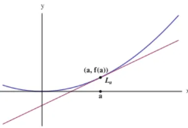
3.2 Local Linear Approximations and the Differential.. . . 122
3.2.1 Local Linear Approximations.. . . 122
3.2.2 The Differential.. . . 128
3.2.3 The Traditional Notation for the Differential.. . . 131
3.2.4 Problems. . . 133
3.3 Rules of Differentiation.. . . 135
3.3.1 The Power Rule. . . 135
3.3.2 Differentiation is a Linear Operation. . . 136
3.3.3 Product and Quotient Rules. . . 138
3.3.4 The Chain Rule. . . 141
3.3.5 The Derivative of an Inverse Function. . . 143
3.3.6 Problems. . . 147
3.4 The Mean Value Theorem. . . 148
3.4.1 The Proof of the Mean Value Theorem.. . . 148
3.4.2 Some Consequences of the Mean Value Theorem. . . 152
3.4.3 Convexity. . . 153
3.4.4 Problems. . . 160
3.5 L’Hôpital’s Rule. . . 161
4 The Riemann Integral. . . 169
4.1 The Riemann Integral.. . . 169
4.1.1 Definition of the Riemann Integral. . . 169
4.1.2 Continuous Functions and Monotone Functions are Integrable.. . . 181
4.1.3 Problems. . . 184
4.2 Basic Properties of the Riemann Integral. . . 185
4.2.1 The Integrals of Combinations of Functions. . . 185
4.2.2 Additivity of the Integral with Respect to Intervals. . . 191
4.2.3 Mean Value Theorems for Integrals. . . 193
4.2.4 Problems. . . 196
4.3 The Fundamental Theorem of Calculus. . . 197
4.3.1 The Fundamental Theorem of Calculus: Part 1. . . 197
4.3.2 The Fundamental Theorem: Part 2. . . 204
4.3.3 Problems. . . 209
4.4 The Substitution Rule and Integration by Parts. . . 210
4.4.1 The Substitution Rule for Indefinite Integrals.. . . 210
4.4.2 The Substitution Rule for Definite Integrals.. . . 213
4.4.3 Integration by Parts for Indefinite Integrals. . . 217
4.4.4 Integration by Parts for Definite Integrals. . . 219
4.4.5 Problems. . . 221
4.5 Improper Integrals: Part 1. . . 222
4.5.1 Improper Integrals on Unbounded Intervals.. . . 222
4.5.2 Improper Integrals That Involve Discontinuous Functions. . . 231
4.5.3 Problems. . . 238
4.6 Improper Integrals: Part 2. . . 239
4.6.1 Comparison Tests for Improper Integrals on Unbounded Intervals. . . 239
4.6.2 Comparison Tests for Improper Integrals That Involve Discontinuous Functions. . . 252
4.6.3 Problems. . . 259
5 Infinite Series. . . 261
5.1 Infinite Series of Numbers. . . 261
5.1.1 Definitions. . . 261
5.1.2 Criteria for the Convergence of Infinite Series. . . 266
5.1.3 Problems. . . 274
5.2 Convergence Tests for Infinite Series: Part 1 . . . 274
5.2.1 The Ratio Test. . . 275
5.2.2 The Root Test. . . 280
5.2.3 The Integral Test. . . 282
5.2.4 Comparison Tests. . . 289
5.2.5 Problems. . . 293
5.3 Convergence Tests for Infinite Series: Part 2 . . . 295
5.3.2 Dirichlet’s Test and Abel’s Test. . . 300
5.3.3 A Strategy to Test Infinite Series for Convergence or Divergence. . . 306
5.3.4 Problems. . . 310
6 Sequences and Series of Functions. . . 313
6.1 Sequences of Functions. . . 313
6.1.1 The Convergence of Sequences of Functions. . . 313
6.1.2 Some Properties of Uniformly Convergent Sequences. . . 320
6.1.3 Proof of Remark 2. . . 327
6.1.4 Problems. . . 329
6.2 Infinite Series of Functions. . . 330
6.2.1 The Convergence of Series of Functions. . . 330
6.2.2 Tests for the Convergence of Series of Functions. . . 331
6.2.3 Continuity, Integrability, and Differentiability of Sums. . . 337
6.2.4 Problems. . . 337
6.3 Power Series. . . 339
6.3.1 The Convergence of Power Series. . . 340
6.3.2 Termwise Integration and Differentiation of Power Series. . . 345
6.3.3 Problems. . . 350
6.4 Taylor Series . . . 351
6.4.1 Taylor’s Formula.. . . 351
6.4.2 Problems. . . 367
6.5 Another Look at Special Functions. . . 369
6.5.1 The Natural Exponential Function.. . . 370
6.5.2 The Natural Logarithm. . . 372
6.5.3 Sine and Cosine. . . 374
Real Numbers, Sequences, and Limits
1.1
Terminology and Notation
In this section we will review some notation and terminology that will be used in this book.
1.1.1
Set Theoretic Terminology and Notation
We will use standard terminology and notation for sets: AsetAis a collection of objects with clearly expressed properties that qualify them for membership inA. We express the fact thatxis an element ofAby writing “x2A” (you can also read this as “xbelongs toA”). For example, the setQof rational numbers is the collection of numbers of the formp=qwherepandqare integers andq¤0. Thus,2=32Q. We can refer toQas
QD fxWxDp=qwherepandqare integers andq¤0g:
When we describe a setAwe need to be clear about the meaning of theequalityof the elements ofA. Equality is a relation between the elements ofAthat satisfies the following conditions:
.i/ xDx
.ii/ IfxDythenyDx(equality is reflexive)
.iii/ IfxDyandyDzthenxDz(equality is transitive).
© Springer International Publishing Switzerland 2016 T. Geveci,Advanced Calculus of a Single Variable, DOI 10.1007/978-3-319-27807-0_1
Thusequality is an equivalence relation. For example, given rational numbers
p1=q1andp2=q2we have
p1
q1 D
p2
q2 if and only ifp1q2Dp2q1:
One may also declare that a rational number is an equivalence class Œp=q
corresponding to the above equivalence relation. In that case we will need to pick a representative from each equivalence class and define the basic arithmetic operations in terms of the representatives. It is more practical to define equality of rational numbers as above and work with them in the way we have since early school years.
SetsAandBareequalif they contain the same elements. In this case we write
ADB. A setAis included in the setB(or, “Ais contained inB”) if each element ofAis also an element ofB. If we use the symbol “)” to denoteimplicationthis fact can be expressed as follows:
x2A)x2B
(this can be read as “ifxis in Athenxis inB”). We will denote the inclusion of the setAinBby writingA B. This notation will not exclude the possibility that
ADB. In some books the notation “AB” is used. If we wish to indicate thatAis contained inBbutAis not equal toBwe will use the notation “A¤B.”
We may use the notation “,” to indicate theequivalenceof statements. Thus “,” can be read as “if and only if.” For example we have
ADB, ABandBA
(“Ais equal toBif and only ifAis contained inBandBis contained onA”). We can abbreviate “if and only if” as “iff.”
Theunionof the setsAandBconsists of elements that belong toAorBand the notation is “A[B.” Thus
A[BD fxWx2Aorx2Bg
(read “the set of allxsuch thatxbelongs toAorxbelongs toB”). The “or” in the above statement is “inclusive or.” It does not exclude the possibility thatxbelongs to bothAandB.
We will indicate the union of an arbitrary collection of sets as
[A2FA:
whereFdenotes that collection. Thus
In particular, ifFconsists of finitely many setsAk,kD 1; 2; : : : ;n, we denote the
union of these sets by
A1[A2[ [Anor [nkD1Ak:
If the collection consists of infinitely many setsAk,kD1; 2; 3; : : :we denote their
union as
A1[A2[: : :Ak[: : : or [1kD1Ak:
Theintersectionof the setsAandBconsists of elements that belong toAandB, and the notation is “A\B.” Thus
A\BD fxWx2Aandx2Bg:
Similarly,
\A2FA
denotes the intersection of the sets in the collectionFso that
\A2FAD fxWx2Afor eachA2Fg:
In particular, ifFconsists of finitely many setsAk,kD 1; 2; : : : ;n, we denote the
intersection of these sets by
A1\A2\ \Anor \nkD1Ak:
If the collection consists of infinitely many setsAk,kD1; 2; 3; : : :we denote their
intersection as
A1\A2\: : :\Ak\: : :or \1kD1Ak:
We will mark the end of a proof by the symbol, the end of an example by, and the end of a remark byÞ.
1.1.2
Functions
Recall that afunctionf from a setUto a setVis a rule that assigns to each element ofUan element ofV. We will denote this by writingf WU !V. The setUis the
domainoff and the setVis thecodomainoff. We will denote the element ofVthat is assigned tou2Uasf.u/. The set all such elements ofVis therangeoff. Thus
In this book we will deal with real-valued functions of a single real variable. We can refer to such a function asf WUR!R. HereRdenotes the set of real numbers andUdenotes the domain off. Thus the codomain off isR. We will denote the range offasf.U/. The graph off is the set of all points in the Cartesian coordinate plane of the form.x;f.x//wherexis in the domain off:
Assume that a functionf is defined so thatf.x/is the same expression for each
xwhere it makes sense. In this case we refer to all suchxas thenatural domain off. For example, iff.x/D pxfor eachx 0the natural domain off is the set of nonnegative real numbers. Ifg.x/D 1=xfor eachx¤ 0the natural domain of
gconsists of all real numbers that are nonzero. We may take a shortcut and refer to
f as “px” and refer togas “1=x.” In such a case, it should be understood that the domain of the relevant function is its natural domain.
Assume thatf andgare both defined on a setUR. We form thesumf Cg
and theproductfgoff andgby performing these operations pointwise: For each
x2U
.f Cg/ .x/Df.x/Cg.x/and .fg/ .x/Df.x/g.x/ :
Thequotient off andgis also defined pointwise: Ifx2Dandg.x/¤0we set
f g
.x/D f.x/ g.x/:
Iff.x/is in the domain ofgfor eachx2Dwe definethe composition off andg
as the functionf ıg(“f composed withg”) such that
.f ıg/ .x/Df.g.x// for eachx2D:
Recall that in generalgıf is different fromfıg(composition is not commutative). For example, iff.x/Dsin.x/for eachx2Randg.x/D1=xfor eachx¤0then
.f ıg/ .x/Df.g.x//Df
1
x
Dsin
1
x
for eachx¤0;
whereas
.gıf/ .x/Dg.f.x//Dg.sin.x//D 1
sin.x/
for eachx 2 Rsuch that sin.x/ ¤ 0, i.e., for eachxthat is not an odd multiple of˙=2.
The trigonometric functionssineandcosineareperiodicwith period2, i.e.
sin.xC2/Dsin.x/and cos.xC2/Dcos.x/ for eachx2R.
The number2is the fundamental period, i.e., the smallest positive period of these functions. The domain of sine and cosine is the set of all real numbersR. Since
1sin.x/1and1cos.x/1for eachx2Rthe range of both functions is the interval
Œ1; 1D fx2RW 1x1/g
Figure1.1displays the graphs of sine and cosine on the intervalŒ2; 2.
Fig. 1.1
2π π2 π 2π
x 1
1y
y = sin(x)
x 1
1y
y =cos(x)
−π
2π −π π2 π 2π
The functiontangentis defined in terms of sine and cosine:
tan.x/D sin.x/
cos.x/if cos.x/¤0:
The fundamental period of tangent is . Since the only points at which cosine vanishes are odd multiples of ˙=2 the domain of tangent consists of all real numbersxsuch that
x¤ ˙.2nC1/
2 for any nonnegative integern:
Fig. 1.2
x
20 10 10 20y
-3p/2 -p -p/2 p/2 p 3p/2
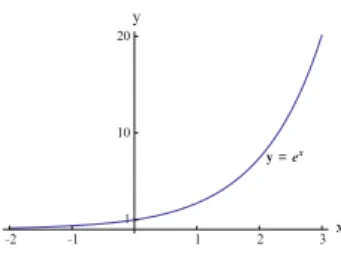
Thenatural exponential function expis defined for all real numbers and attains all positive numbers (Fig.1.3). Usually it is practical to use the exponential notation so that
exp.x/Dex> 0
for eachx2R.
Fig. 1.3 The natural exponential function
2 1 1 2 3x
1 10 20y
y = ex
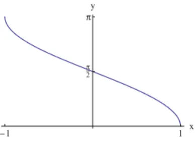
Thenatural logarithmis theinverseof the natural exponential function:
yDln.x/ forx> 0,xDey:
Thus the domain of the natural logarithm is the set of positive real numbers (Fig.1.4).
Fig. 1.4 The natural logarithm
1 2 3 4 5 6 7 x
−2
−3
−4 1 2 y
( e , 1)
e
y = ln(x)
Ifa> 0is an arbitrary base then theexponential function with respect to the baseais defined as
Thelogarithm with respect to the baseais defined so that
yDloga.x/ forx> 0,xDa x:
Thus logarithm with respect to the baseais the inverse of the exponential function with respect to the base. As derived in beginning calculusloga.x/ D ln.
x/ ln.a/ for
eachx> 0:
1.2
Real Numbers
In this section we will summarize the basic rules of arithmetic and the order properties of numbers.
1.2.1
Rules of Arithmetic
The set ofpositive integers (natural numbers)1; 2; 3; : : :will be denoted by N and the set of allintegers
: : : ;3;2;1; 0; 1; 2; 3; : : :
will be denoted byZ.Rational numbersare numbers which can be expressed as fractions of the formp=qwherepandqare integers andq¤0. The set of rational numbers will be denoted byQ. Even though the set of rational numbers is closed under arithmetic operations (sums, products and quotients of rational numbers are also rational numbers), it is not adequate for the purposes of calculus. Indeed, even simple geometric problems lead toirrational numbers,i.e., numbers which are not fractions of integers, as the ancient Greeks knew. For example, the length of the diagonal of a square whose sides are of unit length is the irrational numberp2: The circumference of a circle of unit diameter is the irrational number. We will refer to the set of all rational or irrational numbers as the set ofreal numbersand denote this set byR. We will take it for granted that the setRexists and that the familiar rules for the arithmetic operations of addition, subtraction, multiplication and division are valid: Ifx,y, andzare arbitrary real numbers
1. xCyDyCx(addition is commutative)
2. xC.yCz/D.xCy/Cz(addition is associative)
3. xC0Dx(0 is the additive identity)
4. xC.x/D0(xis the additive inverse: we writexyforxC.y/)
6. x.yz/D.xy/z(multiplication is associative)
7. 1xDx(1 is the multiplicative identity)
8. For eachx¤ 0there exists1=xsuch thatx.1=x/D1:1=xis the multiplicative inverse ofx; we writex=yforx.1=y/
9. x.yCz/DxyCxz(distributive law)
Thus, the set of real numbersRis afield. Note that the set of rational numbersQ is asubfieldofR: When we add, subtract, multiply, or divide fractions of integers we can express the results also as fractions of integers. In the next section we will introduce a crucial property ofRthat is referred to ascompletenessthat is lacking if we stay within the framework ofQ. In the mean time, let us show that the set of rational numbers are inadequate even if we try to compute the square roots of certain integers:
Proposition 1. There is no rational number x such that x2D2:
Proof. Assume that there is such a rational number. We can assume thatx> 0and
xD m n
wheremandnare positive integers. We can also assume that not bothmandnare even since we can cancel any common factor in the numerator and denominator. Now,
x2 D2) m
2
n2 D2)m
2D2n2:
Thusm2is an even positive integer. Ifmwere odd, we could have writtenmas2kC1
for some nonnegative integerkso that
m2D.2kC1/2D4k2C4kC1D22k2C2kC1:
This would have implied thatm2 is odd as well. Thereforemmust be even, say
mD2kfor some positive integerk. Thus
m2D2n2).2k/2D2n2)4k2D2n2)2k2Dn2:
1.2.2
The Order Axioms
Real numbers are equipped with anorder relationship. We write “a<b” to express thatais less thanband we write “a > b” to express thata is bigger thanb. The order relationship has the following properties:
1. Given real numbersaandbexactly one of the relationships
aDb; a<b,a>b
holds.
2. Ifa<bthen for anyc2Rwe haveaCc<bCc(we can add the same number to both sides of an inequality without changing the direction of the inequality).
3. Ifa > 0andb > 0thenab > 0(multiplication of positive numbers yields a positive number).
4. Ifa>bandb>cthena>c(the inequality relationship is transitive).
The above properties lead to the other familiar rules for inequalities. For example,
a>bandc> 0)ac>bc
(when we multiply both sides of an inequality by the same positive number the direction of the inequality is not changed),
a>bandc< 0)ac<bc
(when we multiply both sides of an inequality by the same negative number the direction of the inequality is reversed),
0 <a<b) 1 a >
1
b
(the direction of an inequality between two positive numbers is reversed when we compare their reciprocals)
The notationabmeans thata<boraDb:Similarly,
ab,a>boraDb
Proposition 2. If
a<bC"for each" > 0
then ab. If
a>b"for each" > 0
then ab.
Proof. It is sufficient to prove the first statement. Indeed, if a > b"for each
" > 0thena<bC"for each" > 0:By the first statement we havea b. Thereforeab.
Thus, let us assume that
a<bC"for each" > 0:
We will prove thecontrapositiveof the statement
.a<bC"for each" > 0/)ab:
Thus, we will prove that
a>b)(there exists" > 0such thatabC")
Indeed, if we assume thata>bthen
"D ab 2 > 0:
We have
bC"DbC ab
2 D
aCb
2 <
aCa
2 Da
so thata>bC".
Corollary 1. Ifjabj< "for each" > 0then aDb: Proof. We have
jabj< "for each" > 0,b" <a<bC"for each" > 0:
By Proposition2
abandab:
1.2.3
The Number Line
There is one–one correspondence between the set of real numbers and points on a line. Points on a line are associated with real numbers as follows: A point on the line is selected as the origin. The origin corresponds to 0. Aunit length is selected and the point corresponding to 1 is placed at unit distance from the origin. The origin and the point corresponding to 1 determine the positive direction along the line, and the opposite direction is the negative direction. Usually we place the line horizontally and select the positive direction to the right. If xis a positive number the point corresponding toxis placed at a distancexfrom the origin, in the positive direction. Ifxis a negative number the corresponding point is at the distance
xfrom the origin, in the negative direction. Thus, we establish a correspondence between the set of real numbers and a line. We will refer to the line asthe number lineandidentify the numberxwith the point that corresponds tox. For example, we may refer to “the point2” or “the number 2.” We havea<bif and only ifais to the left ofbon the number line (assuming that the positive direction of the line is towards the right).
Intervals are subsets of the set of real numbers which occur frequently in calculus. Ifa < bthe open interval.a;b/withendpoints a andb is the set of all points betweenaandb:
.a;b/D fx2RWa<x<bg:
We will usually write
.a;b/D fxWa<x<bg;
if it is clear that we are referring to subsets of the set of real numbersR. Note that the open interval.a;b/does not contain the endpointsaandb.
Theclosed intervalŒa;bconsists of the points which lie betweenaandband the endpointsaandbW
Œa;bD fxWaxbg:
We may also considerhalf-open intervalsof the form
Œa;b/D fxWax<bg;
.a;bD fxWa<xbg:
Anunbounded intervalthat consists of all numbers less than a given numberb
is denoted by.1;b/:
There is no need to try to attach a mystical meaning to the symbol1:Within the context of intervals, the symbol merely indicates that the interval contains negative numbers whose distance from the origin is arbitrarily large. Similarly,
.a;C1/D fxWx>ag;
.1;bD fxWxbg;
Œa;C1/D fxWxag:
If J denotes an arbitrary interval, the interior of J is the interval which is obtained by deleting those endpoints of J which belong to J: For example, the interior of the open interval.a;b/coincides with itself, and the interior ofŒa;b/
is the open interval.a;b/.
1.2.4
The Absolute Value and the Triangle Inequality
The absolute value of a number is a measure of the distance of the corresponding point on the number line from the origin:
Definition 1. Ifxis an arbitrary real numberthe absolute value ofxis denoted by
jxjand defined as
jxj D
x ifx0;
xifx< 0:
For example,
j3j D3;
j3j D .3/D3:
Given (real) numbersaandb;we have
jabj D
abifab; baifa<b:
Geometrically,jabjis the distance between the pointsaandbon the number line. For example, the distance between the points 2 and 4 is
j24j D j2j D2;
and the distance between the points 1 and 5 is
Example 1. Let us express the set
AD fxW jx1j 2g
as a union of intervals.
The set A consists of all x whose distance from 1 is at least 2. This means thatx 1 orx 3. Therefore,Ais the union of the intervals .1;1 and
Œ3;C1/, i.e.,
AD.1;1[Œ3;C1/:
We can reach the same conclusion by working with the relevant properties of inequalities:
ifx1thenjx1j Dx1so that
jx1j 2)x12)x3:
Thusx2Œ3;1/:
Ifx< 1thenjx1j D1xso that
jx1j 2)1x2) 1x:
Thusx2.1;1.
ThereforeAD.1;1[Œ3;C1/.
Proposition 3. Assume that r> 0. Then jxj<r if and only ifr<x<r. Simi-larly,jxj r if and only ifrxr.
Proof. Sincejxjis the distance ofxfrom 0 we should havejxj < rif and only if
r<x<r, as in the statement of the proposition. We can reach that conclusion by making use of the relevant properties of inequalities:
Assume thatjxj<r. Ifx0thenxD jxj<r. Sincer> 0we haver< 0x. Thusr<x<r. Ifx< 0thenxD jxj<rso thatx>r. Sincer> 0we have
x< 0 <r. Thusr<x<r.
Conversely, assume thatr <x <r. Ifx 0thenjxj Dx <r. Ifx< 0then
jxj D x<r.
The proof of the second statement is similar.
We will encounter intervals that are described in the following proposition frequently:
Proposition 4. Assume that a2Rand r> 0. We have
Thus,fxW jxaj<rgis the open interval of length2r that is centered at a. We have
fxW jxaj rg DŒar;aCr
so thatfxW jxaj rgis the closed interval of length2r centered at a. Proof. Proposition4is an immediate consequence of Proposition3: We have
jxaj<r, r<xa<r
and
r<xa<r,ar<x<aCr
Thus
fxW jxaj<rg D.ar;aCr/ :
The proof of the second statement is similar.
We will make use of the following fact about the absolute value:
Proposition 5. The absolute value of a product is the product of the absolute values:
jabj D jajjbj:
Proof. We will consider the following cases: 1. a0andb0;
2. a0andb0;
3. a0andb0
4. a0andb0.
In the first case,jaj Da,jbj Db, andab0so that
jabj DabD jaj jbj:
In the second case,jaj Da,jbj D b, andab0so that
jabj D .ab/Da.b/D jaj jbj:
In the third case,jaj D a,jbj Db, andab0so that
In the fourth case,jaj D a,jbj D b, andab0so that
jabj DabD.a/ .b/D jaj jbj:
We will use the triangle inequality frequently:
Theorem 1 (The Triangle Inequality). If a and b are arbitrary real numbers
jaCbj jaj C jbj:
Thus,the absolute value of a sum is less than or equal to the sum of the absolute values.
Proof. SinceaD jajoraD jaj, andbD jbjorbD jbj, we have
jaj a jaj;
jbj b jbj:
Therefore,
jaj jbj aCb jaj C jbj;
i.e.,
.jaj C jbj/aCb jaj C jbj:
IfaCb0,
jaCbj DaCb jaj C jbj:
IfaCb< 0,
.jaj C jbj/aCb) jaj C jbj .aCb/D jaCbj:
Therefore, in all cases,
jaCbj jaj C jbj:
Corollary 2 (Corollary to the Triangle Inequality). If a and b are arbitrary real numbers
Proof. By the triangle inequality,
jaj D jabCbj jabj C jbj;
so that
jaj jbj jabj:
Similarly,
jbj D jbaCaj jbaj C jaj D jabj C jaj;
so that
jbj jaj jabj ) jaj jbj jabj:
Thus,
jabj jaj jbj jabj:
As in the proof of the triangle inequality, the above inequality leads to the inequality
jjaj jbjj jabj:
1.2.5
The Archimedean Property of
R
We will assume theprinciple of mathematical induction:
LetS be a subset of the set of natural numbers N. Assume that N2S and
nC12Sifn2S.Then
SD fn2NWnNg:
In particular, if12Sandn2Simplies thatnC12SthenSDN.
Definition 2. A subsetSofRis said to bewell-ordered(or “has the well-ordering property”) if each nonempty subset ofShas a smallest element.
T consisting of alln 2 T such that1; 2; : : : ;nall belong toT. We will show that
T0 D Nso thatT D Nas well. We have1 2 T0. Assume thatn 2 T0. We need to show thatnC12T0as well. Assume that this is not the case. ThusnC12S. Since
1; 2; : : : ;nall belong toT which is the complement ofS, the numbernC1must be the smallest element ofS. But we have assumed thatSdoes not have a smallest element. ThusnC1 2 T0. ThereforeT0 D N. so thatT D N. ThusS is empty and we have reached a contradiction. ThereforeSmust have a smallest element as claimed.
Definition 3. Assume thatSis a subset ofR. We say thatShas theArchimedean propertyif for eachx2Sthere exists an integernsuch thatx<n:
Note that the set of rational numbersQhas the Archimedean property. Indeed, if
x2Qandx0we can setnD1. Ifx> 0and we expressxasp=qwherepandq
are natural numbers. Then
xD p
q p<pC1:
We will assume that the set of all real numbers has the Archimedean property:
Ifxis an arbitrary real number there exists an integernsuch thatn>x:
Proposition 7. If x and y are positive real numbers there exists a positive integer nsuch that nx>y. In particular, for each positive real number x there exists a positive integer m such that1=m<x.
Proof. By the Archimedean property of real numbers there exists a positive integer
nsuch that
n> y x
Thusnx>y:
In particular, for anyx> 0there exists a positive integermsuch that
mx> 1:
Thusx> 1=m.
1.2.6
Problems
1. Let
AD fx2RW jx1j< 3g
2. Let
AD fx2RW jx2j 6g
ExpressAas an interval.
3. Let
AD fx2RW jx4j> 2g
ExpressAas a union of intervals.
4. Let
AD fx2RWx3 > 4g:
ExpressAas an interval.
5. Let
ADx2RWxC35:
ExpressAas an interval.
6. Assume thatx7. Show that
1
x5
1 2:
7. Assume that3 <x< 4. Show that
3x x1 < 6
8. Assume thatx> 4. Show that
x33x24 > 3
16x3:
9. Assume thatx> 3. Show that
ˇˇ
ˇˇ 2h
.x2/ .xC3/
ˇˇ ˇˇ< 1
3jhj
10. Assume thatx12; x22. Show that
ˇˇ
ˇˇ x2x1
x21.x21/
ˇˇ ˇˇ 1
1.3
The Limit of a Sequence
The concept of the limit is fundamental in calculus. We will begin by discussing the limits of sequences.
1.3.1
The Definition of the Limit of a Sequence
Let us begin by recalling the definition of a sequence:
Definition 1. Asequenceis a function whose domain is a subset of integers of the formfN;NC1;NC2;NC3; : : :g, whereNis a given integer. If we refer to this function asf, thenf.n/is usually denoted asanfornDN;NC1;NC2; : : :.
We may denote asequenceasaN;aNC1;aNC2; : : : ;an; : : :, orfang1nDN, or simply
asfangif we don’t feel the need to specify the starting valueNof theindexn. Thus,
the sequence
1;1 2;
1 3;
1 4; : : : ;
1
n; : : :
can be denoted as
1
n
1
nD1
or
1
n
:
The indexnis a“dummy index” and can be replaced by any other letter. Thus,
1
n
1
nD1
and
1
k
1
kD1
denote the same sequence.
The starting value of the index can be an integer other than 1. For example, if we consider the sequence
5 1;
6 2;
7 3; : : : ;
n n4; : : : ;
the starting value of the index is 5. We can denote the sequence as
n n
n4
o1
nD5.
We may even refer to a sequence simply as “the sequencean.” In this case, it should
expressionan is defined. For example, if we refer to “the sequencen= .n4/” , it
is understood that the starting value ofnis 5. The numberanis referred to asthe
nth termof the sequencea1;a2;a3; : : : ;an; : : :. Thus,1=nis the nth term of the
sequencef1=ng1nD1. In the sequence
5 1;
6 2;
7 3; : : : ;
n n4; : : :
the nth term is not n= .n4/. In such a case we will refer to an as the term
corresponding ton.
The definitions of the graph and the range of a sequence are consistent with the view of a sequence as a function:
Definition 2. The graph of the sequencefang1nDN is the set of points of the form
.n;an/in the Cartesian coordinate plane, wherenDN;NC1;NC2; : : :.The range
of the sequencefang1nDNis the range of the functionf such thatf.n/Dan,nN.
Just as in the case of a function that is defined on an interval, the graph of a sequence helps us visualize the sequence. The graph of a sequence consists of isolated points in the plane, unlike the graph of a function that is defined at all points of an interval. We may also visualize a sequence simply by sketching its range on the number line.
Example 1. Let
anD
n
n4; nD5; 6; 7; : : :
The graph of the sequencefang1nD5is the set of points in the Cartesian coordinate
plane in the form
n; n n4 ;
wheren D 5; 6; 7; : : :. Figure 1.5shows the points in the graph of the sequence corresponding tonD5; 6; 7; : : : ; 20. Figure1.6shows the points in the range of the sequence corresponding tonD5; 6; : : : ; 12.
Fig. 1.5
5 10 15 20x
Fig. 1.6 1 2 3 4 5x
Informally, the limit of the sequencefang1nD1 exists and is the numberLif an
is as close toLas desired provided thatnis sufficiently large. Here is the precise definition:
Definition 3. Thelimit of the sequencefang1nD1isLif for each" > 0there exists
a positive integerNsuch that
janLj< "ifnN:
Example 2. Let
anD
n
n4; nD5; 6; : : : ;
as in Example1. Show that limn!1an D 1(in accordance with the definition of
the limit of a sequence).
Solution. Let" > 0be given. IfnN5then
jan1j Dˇˇˇ
n n4 1
ˇˇ
ˇDˇˇˇˇnnC4
n4
ˇˇ ˇˇD 4
n4
4
N4:
Thus, in order to havejan1j< "fornNit is sufficient to chooseNso that
4
N4 < ":
This is the case if
N4 > 4
" ,N> 4 "C4
Such an integerNexists by the Archimedean property of real number. IfnNthen
jan1j D
4
N4 < ":
Therefore,
lim
n!1anDnlim!1
n n4 D1;
Proposition 1. The limit of a sequence is unique.
Proof. Assume that limn!1an D L1 and limn!1an D L2. We will prove that
L1 D L2by showing thatjL1L2j < "for an arbitrary" > 0. Thus, let" > 0be given. Since limn!1an DL1, there existsN12Nsuch that
nN1 ) janL1j< "
2:
Since limn!1anDL2, there existsN22Nsuch that
nN2 ) janL2j<
" 2:
Therefore, if we setNDmax.N1;N2/then
jaNL1j< "
2 and janL2j< "
2:
Thus,
jL1L2j D j.L1aN/C.aNL2/j jL1aNj C jaNL2j
< " 2C
" 2 D";
with the help of the triangle inequality.
Given a sequencefang1nD1, asubsequenceis formed by selecting those termsan
that correspond to the values of the indexntaken as a strictly increasing sequence: If
n1<n2<n3< <nk<nkC1<
is a strictly increasing sequence of integers the corresponding subsequence of
fang1nD1is
fankg 1
kD1Dan1;an2;an3; : : : ;ank;ankC1; : : :
Example 3. Given the sequence
.1/n1 1
n2
1
nD1
D1;1 22;
1 32;
1 42; ;
Let us set
fnkg1kD1D f2k1g1kD1D1; 3; 5; 7; : : :
so that we will pick those terms that correspond to odd values of the indexn. The corresponding subsequence is
.1/2k 1
.2k1/2
1
kD1
D
1 .2k1/2
1
kD1
D1; 1 32;
1 52;
We can pick those terms that correspond to even values of the indexnby setting
fnkg1kD1D f2kg1kD1D2; 4; 6; 8; : : :
The corresponding subsequence is
.1/2k1 1
.2k/2
1
kD1
D
1 .2k/2
1
kD1
D 1 22;
1 42;
1 62;
Proposition 2. If a sequence converges to L then each subsequence of that sequence converges to the same limit L.
Proof. Assume that
lim
n!1anDL
and that fankg 1
kD1 is a subsequence of fang1nD1. Let " > 0 be given. Since
limn!1anDLthere existsN 2Nsuch that
nN) janLj< ":1
There existsK2Nsuch thatnkNifkK. Thus
kK) jankLj< ":
Therefore limk!1ankDL, as claimed.
Example 4. Show that the sequence
n
sin
n 2
o1
nD1
does not have a limit.
Solution. Let’s see what the first few terms of the sequence look like:
sin
2 ;sin./ ;sin
3 2
;sin.2/ ;sin
5 2 ;sin 6 2 ;sin 7 2 ;sin 8 2 ;sin 9 2 ; : : : i.e.
1; 0;1; 0; 1; 0;1; 0; 1; : : :
We have
sin
.nC4/
2 Dsin
n
2 C2 Dsin
n
Thus, the pattern1; 0;1; 0is repeated. The sequences
1; 1; 1; 1; : : : 0; 0; 0; 0; : : : 1;1;1;1; : : :
are subsequences of the given sequence and have the limits 1, 0, and1, respec-tively. Since we displayed subsequences with different limits, the sequence does not have a limit.
1.3.2
The Limits of Combinations of Sequences
Now we will establish the rules about the limits of certain combinations of sequences. These rules are intuitively plausible and you must have been using them since beginning Calculus. Here we will provide rigorous proofs.
Proposition 3. The limit of a constant sequence c is c.
Proof. Assume thatan Dcfor eachn2N. We need to show that limn!1an Dc.
Let" > 0be given. We have
jancj D jccj D0 < "
for eachn1. Therefore, limn!1anDc.
Proposition 4 (The Constant Multiple Rule for Limits). Assume that c is a constant andlimn!1anexists. Then
lim
n!1.can/Dcnlim!1an:
Proof. IfcD0thencanD0for eachnso that
lim
n!1.can/Dnlim!1.0/D0:
Thus, let us assume thatc¤0and that limn!1an DL. Let" > 0be given. Since
limn!1anDLthere existsN 2Nsuch that
nN) janLj< "
jcj:
Then,
jcancLj D jc.anL/j D jcj janLj<jcj
" jcj
Therefore,
lim
n!1.can/DcLDcnlim!1an;
as claimed.
Proposition 5 (The Sum Rule for Limits). Assume that limn!1an and
limn!1bnexist. Thenlimn!1.anCbn/exists and
lim
n!1.anCbn/Dnlim!1anCnlim!1bn:
Proof. Let limn!1anDAand limn!1bnDBand let" > 0be given. There exists
N12NandN22Nsuch that
nN1) janAj<
"
2 andnN2) jbnBj<
" 2
SetNDmax.N1,N2/. IfnNwe have
j.anCbn/.L1CL2j D j.anL1/C.bnL2/j
janL1j C jbnL2j
< " 2 C
" 2 D":
Therefore
lim
n!1.anCbn/DL1CL2Dnlim!1anCnlim!1bn
as claimed.
Proposition 6. A convergent sequence is bounded.
Proof. Assume that limn!1an exists. We need to show that there existsM > 0
such thatjanj Mfor eachn2N.
Assume that limn!1anDL. There existsN2Nsuch that
nN) janLj< 1:
Therefore, ifnNthen
janj D j.anL/CLj janLj C jLj< 1C jLj:
Set
MDmax.ja1j;ja2j; : : :I jaN1j; 1C jLj/ :
Proposition 7 (The Product Rule for Limits). Assume that limn!1an and
limn!1bnexist. Then
lim
n!1anbnD
lim
n!1an
lim
n!1bn
(the limit of a product is the product of the limits).
Proof. Let limn!1an DL1and limn!1bnDL2. We need to show that
lim
n!1anbnDL1L2:
We have
janbnL1L2j D janbnL1bnCL1bnL1L2j
D j.anL1/bnCL1.bnL2/j
janL1j jbnj C jL1j jbnL2j;
thanks to the triangle inequality.
Since a convergent sequence is bounded, there existsM> 0such thatjbnj M
for eachn2N. Therefore,
janbnL1L2j janL1j jbnj C jL1j jbnL2j
MjanL1j C jL1j jbnL2j:
Let" > 0be given. Since limn!1anDL1and limn!1bnDL2, there existsN2N
such that
nN) janL1j<
"
2 .MC jL1j C1/ and jbnL2j<
"
2 .MC jL1j C1/:
Thus, ifnNthen
janbnL1L2j MjanL1j C jL1j jbnL2j
<M
" 2 .MC jL1j C1/
C jL1j
" 2 .MC jL1j C1/
D
M
.MC jL1j C1/
"
2 C
j
L1j
.MC jL1j C1/
" 2 < "
2 C " 2 D":
Proposition 8 (The Quotient Rule for Limits). Assume that limn!1an and
limn!1bnexist andlimn!1bn. Then
lim
n!1
an
bn
D limn!1an
limn!1bn
Proof. By Proposition7on the limit of a product, it is sufficient to show that
lim
n!1
1
bn
D 1
limn!1bn
;
provided that limn!1bn¤0. Let limn!1bnDL¤0. We need to show that
lim n!1 1 bn D 1 L: We have ˇˇ ˇˇb1n 1
L
ˇˇ
ˇˇDˇˇˇˇLbn
bnL
ˇˇ
ˇˇD jbnLj
jbnj jLj
:
Since limn!1bnDL¤0, there existsN12Nsuch that
nN1) jbnLj<
jLj
2 :
Then
jbnj D jL.Lbn/j jLj jLbnj>jLj
jLj
2 D
jLj
2 ;
thanks to the corollary to the triangle inequality. Thus,
ˇˇ ˇˇb1n 1
L
ˇˇ
ˇˇD jbnLj
jbnj jLj <
jbnLj
j
Lj
2
jLj
D 2
L2
jbnLj
ifnN1.
Let" > 0be given. Since limn!1bn DL¤0there existsNN1such that
jbnLj<
L2
2
"
ifnN. Then,
ˇˇ ˇˇb1n 1
L ˇˇ ˇˇ< 2 L2
jbnLj<
2 L2 L2 2
"D":
Proposition 9. Assume that an<bnfor each n andlimn!1anand limn!1bnexist.
Then
lim
n!1annlim!1bn:
Proof. Let limn!1an DL1and limn!1bn DL2. We need to show thatL1 L2.
We will achieve this by showing that
L1<L2C"
for each" > 0.
Thus, let" > 0be arbitrary. Since limn!1an DL1and limn!1bnDL2, there
existsN2Nsuch that
janL1j<
"
2 andjbnL2j<
" 2
ifnN. Therefore,
L1L2D.L1aN/C.aNbN/C.bNL2/
jL1aNj .bNaN/C jbnL2j
<jL1aNj C jbNL2j;
sincebNaN> 0. Thus
L1L2<jL1aNj C jbNL2j<
" 2 C
" 2 D";
so that
L1<L2C":
Corollary 1. Assume that an<M for each n andlimn!1anexists. Then
lim
n!1anM:
Proof. Corollary1follows immediately from Proposition9since limn!1MDM.
Remark 1. We cannot claim that limn!1an < M if an < M for each n. For
example,
11
for eachn, but
lim
n!1
11
n
D1:
Þ
1.3.3
Problems
In problems1–6,
a) Determine the limit of the given sequencefang(as in elementary calculus).
b) Justify your assertion in accordance with the definition of the limit of a sequence.
1.
anD
1
2n3; nD2; 3; 4; : : :
2.
anD
4n3
nC9; nD1; 2; 3; : : :
3.
anD
3n2C1
n2C4 ; 1; 2; 3; : : :
4.
anD
n
n22; nD2; 3; 4; : : :
5.
anD
n
2nCpn; nD1; 2; 3; : : :
6.
anD
p
nC1pn; nD1; 2; 3; : : :
7. Prove that
lim
n!1
sin.10n/
p
n D0
in accordance with the definition of the limit of a sequence.
8. Assume thatjaj< 1. Prove that
lim
n!1a
nD0:
9. Prove “the squeeze theorem”:
Assume thatcn anbnfor eachn2Nand
lim
n!1cnDnlim!1bnDL:
Then limn!1anexists and
lim
n!1anDL:
10. Show that
1
3 Dnlim!1
3 10C
3 102 C
3
103 C C
3 10n
:
(you need not use the"Ndefinition of the limit). Hint: Make use of the identity
1CxCx2C Cxn D 1x
n
1x ifx¤1:
1.4
The Cauchy Convergence Criterion
In this section we will discuss theCauchy convergence criterionfor the conver-gence of a sequence. The criterion enables us to predict that the sequence has a limit even if we have no prior knowledge about the exact value of its limit. We will use the Cauchy convergence criterion extensively in the following chapters.
1.4.1
Basic Facts about Cauchy Sequences
Definition 1. A sequencefang1nD1is aCauchy sequenceif, given any" > 0, there
existsN2Nsuch that
Remark 1. We can setmDnCk,kD1; 2; 3; : : :and state the fact that a sequence
fang1nD1 is a Cauchy sequence in the following alternative form: Given any" > 0
there existsN2Nsuch that
nN) jananCkj< "forkD1; 2; 3; : : :
Intuitively, a sequence satisfies the Cauchy condition if its terms are arbitrarily close to each other provided that they correspond to indices that are sufficiently large, no matter how far apart they may be.Þ
Proposition 1. A sequence that converges is a Cauchy sequence.
Proof. Assume that limn!1anDL. For a given" > 0there existsN2Nsuch that
janLj< "
2 ifnN:
IfnNandmNthen
janamj D j.anL/C.Lam/j janLj C jamLj< "
2C " 2 D":
Afinite decimal is an expression of the forma0:a1a2a3: : :an. Herea0 is an
integer andan2 f0; 1; 2; : : : ; 9g. The corresponding rational number is
a0C a101 C10a22 C 10a33 C C10ann
Aninfinite decimala0:a1a2a3: : :an: : :is shorthand for
lim
n!1
a0C a1
10C
a2
102 C
a3
103C C
an
10n :
If a block of digits is repeated indefinitely the limit is a rational number as in the following example:
Example 1. We have
1
2 D0:4999 : : : ; 1
3 D0:33333 : : :
Let us confirm that
1
2 D0:4999 : : :
We will use the identity
1CxCx2C CxnD 1x
nC1
1x ifx¤1
(check). We have
4 10C
9 102 C
9
103 C C
9 10n D
4 10C
9 102
1C 1
10 C 1
102 C C
1 10n2
D 4 10C 9 102 0 B @1 1 10n1
1 1
10 1 C A D 4 10C 1 10
1 1
10n1
: Therefore lim n!1 4 10C 9 102 C
9
103 C C
9 10n D lim n!1 4 10 C 1 10
1 1
10n1
D 4 10C 1 10D 5 10 D 1 2: Thus 1
2 D0:4999 : : : :
We can show that a sequence that corresponds to an infinite decimal is a Cauchy sequence, even if the limit cannot be determined as in the above cases:
Proposition 2. Given the infinite decimal
a0:a1a2a3: : :an: : :
the sequencefSng1nD1where
SnDa0C
a1
10C
a2
102 C
a3
103 C C
an
10n
Proof. IfkD1; 2; 3; : : :, we have
0SnCkSnD
anC1
10nC1C
anC2
10nC2 C
anC3
10nC3 C C
anCk
10nCk
9 10nC1C
9 10nC2 C
9
10nC3 C C
9 10nCk
D 9 10nC1
1C 1
10C 1
102 C C
1 10k1
9 10nC1
0 B @1
1 10k
1 1
10 1 C AD 1
10n
1 1
10k
< 1
10n:
Thus, given" > 0we can chooseN2Nso that
1
10N < ",
1 " < 10
N:
IfnNandkD1; 2; 3; : : :we have
0SnCkSn< 1
10n
1 10N < ":
ThereforefSng1nD1is a Cauchy sequence.
Does such a Cauchy sequencefSng1nD1converge to a real number? Let us pose
the question in a more general framework: Does any Cauchy sequence of numbers converge to a real number?We will accept the following statement as an axiom:
The Cauchy Convergence Principle:
A Cauchy sequence of real numbers converges to a real number.
In particular, any decimala0:a1a2a3: : :an: : :represents a real numberxin the
sense that the Cauchy sequence
SnDa0C
a1
10C
a2
102 C
a3
103 C C
an
10n
converges tox.
Remark 2. Assume that we have shown that fxng1nD1 is a Cauchy sequence by
determining an integerN"such