Introducci ´on al Aprendizaje de M ´aquina
Hernán Felipe García Arias M.Sc. Aprendizaje de Máquina Universidad del Quindío
Contenido
Introducci ´on
Definiciones
An ´alisis de Patrones
Teor´ıa de la probabilidad
Teor´ıa de decisi ´on
Aprendizaje de M ´aquina ´o Aprendizaje Estad´ıstico
q El aprendizaje de m ´aquina o aprendizaje estad´ıstico juega un papel clave en direferentes ´areas de la ciencia, la ingenier´ıa, las finanzas o la industria.
q Algunos ejemplos de problemas de aprendizaje son
– Predecir si un paciente, hospitalizado por un infarto, tendr ´a un segundo infarto. La predicci ´on debe hacerse con base en medidas cl´ınicas, demogr ´aficas y de dieta del paciente.
– Predecir el precio de un acci ´on, a seis meses de hoy, usando como base mediciones sobre el desempe ˜no de la compa ˜n´ıa, y datos econ ´omicos.
– Identificar los n ´umeros de un c ´odigo postal escrito a mano, a partir de una imagen digitalizada.
– Estimar la cantidad de glucosa en la sangre de una persona diab ´etica, a partir del espectro de absorci ´on infrarroja de la sangre de la persona.
Aprendizaje de M ´aquina ´o Aprendizaje Estad´ıstico
q Este curso es sobreaprendizaje a partir de datos.
q En un escenario t´ıpico, se tiene una medida de salida, usualmente cuantitativa (como el precio de una acci ´on en la bolsa) o categ ´orica (como infarto/no infarto), que se desea predecir, con base en un conjunto decaracter´ısticas(como las medidas cl´ınicas o de dieta).
q Se parte de un conjunto de los datos, conocido comoconjunto de entrenamiento, en el cual se observan las salidas y las caracter´ısticas de un conjunto de objetos (por ejemplo, personas).
q Usando estos datos se construye un modelo de predicci ´on, o un aprendiz, que permite predecir la salida correspondiente a un conjunto de caracter´ısticas asociadas a un nuevo objeto que no se ha visto con anterioridad.
Ejemplo 1: Detecci ´on de Spam (I)
q Se tiene informaci ´on de 4601 correos electr ´onicos.
q Se desea predecir si un correo electr ´onico es spam, antes de llenar el inbox de un usuario.
q Para los 4601 correos, se conoce la verdadera variable de salida (si es email ´o spam).
q As´ı mismo se conoce las frecuencias relativas de 57 de las palabras que ocurren con mayor frecuencia.
Ejemplo 1: Detecci ´on de Spam (II)
q Porcentajes promedio de palabras y caracteres en un correo electr ´onico.
george you your hp free hpl ! our re edu remove spam 0.00 2.26 1.38 0.02 0.52 0.01 0.51 0.51 0.13 0.01 0.28 email 1.27 1.27 0.44 0.90 0.07 0.43 0.11 0.18 0.42 0.29 0.01
q El m ´etodo de aprendizaje deber´ıa seleccionar cu ´ales caracter´ısticas usar y c ´omo.
q Por ejemplo
– Si(%george<0.6)y(%you>1.5)es spam, de lo contrario es email. – Si(0.2×%you−0.3×%george>0)es spam, de lo contrario es email.
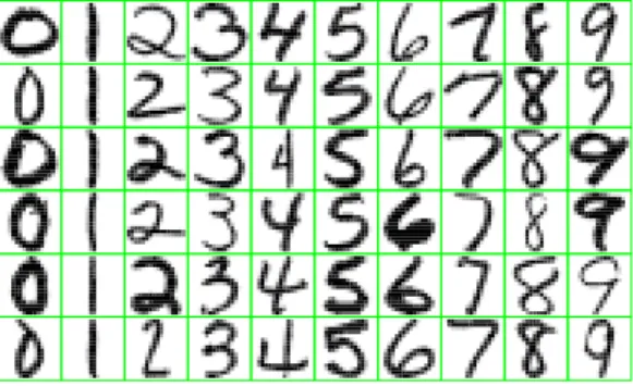
Ejemplo 2: D´ıgitos manuscritos
Elements of Statistical Learning (2nd Ed.) cHastie, Tibshirani & Friedman 2009 Chap 1
FIGURE 1.2. Examples of handwritten digits from U.S. postal envelopes.
q Cada imagen es un segmento de c ´odigo postal de 5 d´ıgitos. q Las im ´agenes tienen dimensiones de 16×16 pixeles, en escala de
grises. La intensidad de cada pixel se encuentra en el rango de 0 a 255.
Contenido
Introducci ´on
Definiciones
An ´alisis de Patrones
Teor´ıa de la probabilidad
Teor´ıa de decisi ´on
Definiciones b ´asicas
q Conjunto de entrenamiento(X): conjunto deNd´ıgitos{x1, . . . ,xN}
empleados para sintonizar los par ´ametros de un modelo de predicci ´on.
q Vector de etiquetas(t): las categor´ıas de los d´ıgitos en el conjunto de entrenamiento se conocen de antemano.
q Entrenamiento: el resultado de ejecutar el algoritmo de aprendizaje de m ´aquina puede ser expresado como una funci ´ony(x)que toma un d´ıgitoxy entrega una salida codificada de la misma manera quet.
q Validaci ´on: probar la funci ´on obtenida con un conjunto diferente de d´ıgitos a los utilizados en el entrenamiento (conjunto de validaci ´on).
q Generalizaci ´on: habilidad de clasificar correctamente d´ıgitos de
Aprendizaje supervisado y no supervisado
q Aprendizaje supervisado: se conocen los vectores de caracter´ısticas (X), y sus correspondientes etiquetas de salida (t).
– La variable de salida es discreta:clasificaci ´on. – La variable de salida es continua:regresi ´on.
q Aprendizaje no supervisado: s ´olo se conocen los vectores de caracter´ısticas (X)
– Descubrir grupos de datos similares:agrupamiento.
– Determinar la distribuci ´on de los datos:estimaci ´on de densidad. – Proyectar los datos a un espacio de menor dimensi ´on:reducci ´on de
dimensionalidad.
q Otro tipo de aprendizaje: semi-supervisado, aprendizaje activo,
Contenido
Introducci ´on
Definiciones
An ´alisis de Patrones
Teor´ıa de la probabilidad
Teor´ıa de decisi ´on
Ejemplo Regresi ´on (I)
x t
0 1
−1 0 1
q Regresi ´on: supongamos una funci ´on conocida sen(2πx)con ruido aleatorio incluido en la variable objetivot.
Ejemplo Regresi ´on (II)
q Objetivo: usar el conjunto de entrenamiento para hacer prediccionesˆt
para alg ´un valor nuevo deˆx.
q Dificultad: generalizar sen(2πx)a partir de un conjunto finito de datos.
Funci ´on polinomial (I)
q Usando como modelo de predicci ´on una funci ´on polinomial,
y(x,w) =w0+w1x+. . .+wMxM= M X
j=0 wjxj,
dondew≡ {w0,w1, . . . ,wM}.
q N ´otese que la funci ´on es lineal respecto aw.
q El proceso de entrenamiento consiste en encontrar los coeficientesw,
Funci ´on polinomial (II)
q Esto se realiza minimizando una funci ´on de error
E(w) =1
2
N X
n=1
{y(xn,w)−tn}2.
q La minimizaci ´on del error tiene soluci ´on ´unicaw∗. El polinomio resultante estar ´a dado pory(x,w∗).
t
x y(xn,w) tn
Selecci ´on del modelo
Una pregunta natural: c ´omo escoger el orden del polinomio,M?
x t
M= 0
0 1 −1 0 1 x t
M= 1
0 1 −1 0 1 x t
M= 9
0 1 −1 0 1 x t
M= 3
0 1
Validaci ´on
q Para lograr una buena generalizaci ´on, verificarE(w∗)sobre un
conjunto de validaci ´on usando
ERMS= p
2E(w∗)/N.
q El error RMS permite comparar errores para conjuntos de diferentes tama ˜nos.
M
ER
M
S
0 3 6 9
0 0.5 1
Modelo en funci ´on de
N
(
M
=
9).
x t
N= 15
0 1
−1 0 1
x t
N= 100
0 1
−1 0 1
Regularizaci ´on (I).
x t
M= 9
0 1
−1 0 1
1.1. Example: Polynomial Curve Fitting 11
Table 1.2 Table of the coefficientswforM= 9polynomials with various values for the regularization parameterλ. Note thatlnλ = −∞corresponds to a model with no regularization, i.e., to the graph at the bottom right in Fig-ure 1.4. We see that, as the value of λincreases, the typical magnitude of the coefficients gets smaller.
lnλ=−∞ lnλ=−18 lnλ= 0 w
0 0.35 0.35 0.13
w
1 232.37 4.74 -0.05 w
2 -5321.83 -0.77 -0.06 w
3 48568.31 -31.97 -0.05 w
4 -231639.30 -3.89 -0.03 w
5 640042.26 55.28 -0.02 w
6 -1061800.52 41.32 -0.01 w
7 1042400.18 -45.95 -0.00 w
8 -557682.99 -91.53 0.00 w
9 125201.43 72.68 0.01
the magnitude of the coefficients.
The impact of the regularization term on the generalization error can be seen by plotting the value of the RMS error (1.3) for both training and test sets againstlnλ, as shown in Figure 1.8. We see that in effectλnow controls the effective complexity of the model and hence determines the degree of over-fitting.
The issue of model complexity is an important one and will be discussed at length in Section 1.3. Here we simply note that, if we were trying to solve a practical application using this approach of minimizing an error function, we would have to find a way to determine a suitable value for the model complexity. The results above suggest a simple way of achieving this, namely by taking the available data and partitioning it into a training set, used to determine the coefficientsw, and a separate validationset, also called ahold-outset, used to optimize the model complexity (eitherM orλ). In many cases, however, this will prove to be too wasteful of valuable training data, and we have to seek more sophisticated approaches.
Section 1.3
So far our discussion of polynomial curve fitting has appealed largely to in-tuition. We now seek a more principled approach to solving problems in pattern recognition by turning to a discussion of probability theory. As well as providing the foundation for nearly all of the subsequent developments in this book, it will also
Figure 1.8 Graph of the root-mean-square er-ror (1.3) versuslnλfor theM= 9
polynomial.
ERM
S
lnλ
−35 −30 −25 −20
0 0.5 1
Training Test
Se puede regularizar la funci ´on de error para prevenir quewtome valores grandes
E(w) =1
2
N X
n=1
{y(xn,w)−tn}2+λ
2kwk
2,
dondeλes el t ´ermino de regularizaci ´on.
Regularizaci ´on (II).
x t
lnλ=−18
0 1 −1 0 1 x t
lnλ= 0
0 1
−1 0 1
1.1. Example: Polynomial Curve Fitting 11
Table 1.2 Table of the coefficientswforM= 9polynomials with various values for the regularization parameterλ. Note thatlnλ = −∞corresponds to a model with no regularization, i.e., to the graph at the bottom right in Fig-ure 1.4. We see that, as the value of λincreases, the typical magnitude of the coefficients gets smaller.
lnλ=−∞ lnλ=−18 lnλ= 0
w
0 0.35 0.35 0.13
w
1 232.37 4.74 -0.05 w
2 -5321.83 -0.77 -0.06 w
3 48568.31 -31.97 -0.05 w
4 -231639.30 -3.89 -0.03 w
5 640042.26 55.28 -0.02 w
6 -1061800.52 41.32 -0.01 w
7 1042400.18 -45.95 -0.00 w
8 -557682.99 -91.53 0.00 w
9 125201.43 72.68 0.01
the magnitude of the coefficients.
The impact of the regularization term on the generalization error can be seen by plotting the value of the RMS error (1.3) for both training and test sets againstlnλ, as shown in Figure 1.8. We see that in effectλnow controls the effective complexity of the model and hence determines the degree of over-fitting.
The issue of model complexity is an important one and will be discussed at length in Section 1.3. Here we simply note that, if we were trying to solve a practical application using this approach of minimizing an error function, we would have to find a way to determine a suitable value for the model complexity. The results above suggest a simple way of achieving this, namely by taking the available data and partitioning it into a training set, used to determine the coefficientsw, and a separate validationset, also called ahold-outset, used to optimize the model complexity (eitherM orλ). In many cases, however, this will prove to be too wasteful of valuable training data, and we have to seek more sophisticated approaches.
Section 1.3
So far our discussion of polynomial curve fitting has appealed largely to in-tuition. We now seek a more principled approach to solving problems in pattern recognition by turning to a discussion of probability theory. As well as providing the foundation for nearly all of the subsequent developments in this book, it will also
Figure 1.8 Graph of the root-mean-square er-ror (1.3) versuslnλfor theM= 9
polynomial. ERM S 0 0.5 1 Training Test
Contenido
Introducci ´on
Definiciones
An ´alisis de Patrones
Teor´ıa de la probabilidad
Teor´ıa de decisi ´on
Teor´ıa de la probabilidad
Lateor´ıa de la probabilidades la herramienta que usamos para cuantificar el nivel de incertidumbre que se tiene sobre el problema de aprendizaje.
Teorema de Bayes en Aprendizaje de M ´aquina
q Para el caso de aprendizaje de m ´aquina,D={t1, . . . ,tN},
p(w|D) = p(D|w)p(w) p(D) .
q Posterior:p(w|D).
q Verosimilitud:p(D|w).
q A-priori:p(w).
q Evidencia:p(D) =R
Aplicaci ´on teor´ıa de probabilidad en regresi ´on (I)
q Retomando el problema de regresi ´on, se tienenx={x1, . . . ,xN}>, t={t1, . . . ,tN}>.
q Se asume el siguiente modelo probabil´ıstico para los datos
t =y(x,w) +,
dondesigue una distribuci ´on Gaussian∼ N(0, β−1).
q Esto significa que siβ ywfuesen conocidos, la variable de salida seguir´ıa
p(t|x,w, β) =N(t|y(x,w), β−1),
Aplicaci ´on teor´ıa de probabilidad en regresi ´on (II)
t
x x0
2σ
y(x0,w)
y(x,w)
p(t|x0,w, β)
q Suponiendo que los datos soniid
p(t|x,w, β) = N Y
n=1
N(tn|y(xn,w), β−1).
Teor´ıa de estimaci ´on en Aprendizaje de M ´aquina
q La teor´ıa de estimaci ´on estad´ıstica puede emplearse para encontrar los par ´ametroswyβ, del modelo de predicci ´on.
q M ´axima verosimilitud (maximizando la funci ´on de verosimilitud
logar´ıtmica).
q Inferencia Bayesiana (asumiendo alguna forma para la funci ´on a-priori
Contenido
Introducci ´on
Definiciones
An ´alisis de Patrones
Teor´ıa de la probabilidad
Teor´ıa de decisi ´on
M´ınimo Error de Clasificaci ´on (I)
q Frontera de decisi ´on. RegionesRk → Ck en las que se divide el
espacio de entrada por medio de la regla de decisi ´on parax.
q La probabilidad de error est ´a dada como
p(error) =p(x∈ R1,C2) +p(x∈ R2,C1)
= Z
R1
p(x,C2)dx+ Z
R2
p(x,C1)dx.
q Sip(x,C1)>p(x,C2)para unxdado, se debe elegirC1.
M´ınimo Error de Clasificaci ´on (II)
R1 R2
x0
b x
p(x,C1)
p(x,C2)
M´ınimo Error de Clasificaci ´on: K clases
q ParaK clases se maximiza la probabilidad de estar en lo correcto,
p(correcto) = K X
k=1
p(x∈ Rk,Ck) = K X
k=1 Z
Rk
p(Ck|x)p(x)dx.
q La observaci ´onxse asigna a la clase que tenga mayorp(Ck|x).
P ´erdida esperada m´ınima (I)
q Funci ´on de p ´erdida. Medida de la p ´erdida en que se incurre al tomar una decisi ´on equivocada, L.
q Objetivo. Minimizar la p ´erdidad total.
q Por ejemplo, se tiene la siguiente matriz de p ´erdida c ´ancer normal c ´ancer 0 1000 normal 1 0
q La soluci ´on ´optima es aquella que minimiza la funci ´on de p ´erdida.
P ´erdida esperada m´ınima (II)
q Como se conocep(x,Ck)se puede minimizar la p ´erdida esperada,
E(L) = X k X j Z Rj
Lkjp(x,Ck)dx= X k X j Z Rj
Lkjp(Ck|x)p(x)dx.
q El objetivo es escoger las regionesRj que minimicen la p ´erdida
esperada.
q Para una entrada particularxse debe minimizarP
kLkjp(x,Ck).
q Regla de decisi ´on. Asignar cada nuevoxa la clasejpara la cual la cantidad
X
k
Lkjp(x,Ck),
Opci ´on de rechazo
Evitar tomar decisiones dif´ıciles, introduciendo un umbralθ.
x p(C1|x) p(C2|x)
0.0 1.0
θ
Inferencia y decisi ´on (I)
q Clasificaci ´on en dos etapas: inferencia y decisi ´on.
q Tres enfoques distintos.
q Modelos generativos.
– Determinar primerop(x,Ck)para obtenerp(Ck|x).
– Luego usar teor´ıa de la informaci ´on para elegir la clase de cada observaci ´onx.
q Modelos discriminativos.
– Determinar directamentep(Ck|x).
– Luego usar teor´ıa de la informaci ´on para elegir la clase de cada observaci ´onx.
q Funci ´on discriminante.f(x)es un mapeo directo de la observaci ´onx
Inferencia y decisi ´on (II)
p(x|C1)
p(x|C2)
x
class densities
0 0.2 0.4 0.6 0.8 1 0
1 2 3 4 5
x
p(C1|x) p(C2|x)
0 0.2 0.4 0.6 0.8 1 0
Funci ´on de p ´erdida: regresi ´on (I)
q Regresi ´on: estimary(x)para el correspondientetde la entradax.
q Supongamos que se incurre en una p ´erdidaL(t,y(x)).
q El valor esperado de la p ´erdida est ´a dado como
E(L) =
Z Z
L(t,y(x))p(x,t)dxdt.
q Si la funci ´on de p ´erdida es cuadr ´atica, se tiene
E(L) =
Z Z
{t−y(x)}2p(x,t)dxdt.
Funci ´on de p ´erdida: regresi ´on (II)
q Asumiendo quey(x)es totalmente flexible, y utilizando c ´alculo de variaciones
∂E(L)
∂y(x) =−2 Z
{t−y(x)}p(x,t)dt.
q Igualando a cero y despejandoy(x)
y(x) = R
t p(x,t)dt p(x) =
Z
t p(t|x)dt =Et[t|x].
Funci ´on de p ´erdida: regresi ´on (III)
t
x x0
y(x0)
y(x)
Funci ´on de p ´erdida: regresi ´on (IV)
Como en clasificaci ´on, el problema de regresi ´on se puede resolver con tres enfoques diferentes
q M ´etodo generativo
– Encontrarp(x,t), y luegop(t|x). – CalcularEt[t|x].
q M ´etodo discriminativo
– Encontrar directamentep(t|x). – CalcularEt[t|x].
Otras funciones de p ´erdida
La p ´erdida de Minkowski est ´a dada como|y(x)−t|q.
y−t
| y − t | q
q= 0.3
−2 −1 0 1 2
0 1 2
y−t
| y − t | q
q= 1
−2 −1 0 1 2
0 1 2
y−t
| y − t | q
q= 2
−2 −1 0 1 2
0 1 2
y−t
| y − t | q
q= 10
−2 −1 0 1 2
Contenido
Introducci ´on
Definiciones
An ´alisis de Patrones
Teor´ıa de la probabilidad
Teor´ıa de decisi ´on
Selecci ´on del modelo
q Definici ´on. Seleccionar los par ´ametros del modelo que produzcan mayor generalizaci ´on.
q Gran cantidad de datos→validaci ´on hold out.
q Pocos datos→validaci ´on cruzada o leave-one-out.