BIBLIOTECA
This work is licensed under a
Creative Commons Attribution-NonCommercial-NoDerivatives
4.0 International License.
Document downloaded from the institutional repository of the University
of Alcala:
http://dspace.uah.es/dspace/
This is a postprint version of the following published document:
Ferrari, M., et al., 2016, "Analysis of Bundles and Drivers of Change of
Multiple Ecosystem Services in an Alpine Region",
Journal of
Environmental Assessment Policy and Management,
vol. 18, no. 04, pp.
1650026.
Available at
http://dx.doi.org/10.1142/S1464333216500265
© 2016 World Scientific Publishing
Journal of Environmental Assessment Policy and Management
Analysis of bundles and drivers of change of multiple ecosystem services in an Alpine
region
--Manuscript
Draft--Manuscript Number: JEAPM-D-16-00061R1
Full Title: Analysis of bundles and drivers of change of multiple ecosystem services in an Alpine
region
Article Type: Research Paper
Keywords: Ecosystem services; bundles; drivers of change; principal components; cluster
analysis; Alpine region
Corresponding Author: marika ferrari, Ph.D.
ITALY
Corresponding Author Secondary Information:
Corresponding Author's Institution:
Corresponding Author's Secondary Institution:
First Author: marika ferrari, Ph.D.
First Author Secondary Information:
Order of Authors: marika ferrari, Ph.D.
Davide Geneletti, associated professor
Luis Cayuela, associated professor
Jose María Rey Benayas, full professor
Francesco Orsi, Assistant professor
Order of Authors Secondary Information:
Abstract: Approaches based on the concept of the ecosystem services need analyses of the
sets of spatially correlated services (i.e. bundles) and of the external factors that modify the ecosystem service supply (i.e. drivers of change). At present, appropriate methods to analyze bundles and drivers of change are still under development.
This study proposes a method based on a combination of spatial and statistical analyses to define bundles and to explain the drivers of change of 24 ecosystem services in Trentino, an Alpine region of Italy. Results show that multiple services can be grouped in a few number of bundles with a complex shape. When mapping multiple services across the territory, the spatial units of representation are a combination of the intrinsic units of representation of single ecosystem services and land use classes. Land use management was found as the external factor that causes the greatest variability of the ecosystem services distribution across the region.
Response to Reviewers:
MANUSCRIPT
From line 100 to line 110: I inserted the explanation for PCA as requested
In inserted the minor edits:
*Abstract: When mapping multiple services...a combination the metric units...-change to a combination "of" metric units
*line 18 First there is not general agreement.... - change "not" to "no"
*line 34 Maes et al (2011b) considered the supply of 13 sevices for all Europe ...-change "all" Europe to "the whole of" Europe
*line 36 bundles definition - change "bundles" to "bundles'"
*line 46 the region ...above "sea level" - change to "above sea level (a.s.l)" *line 84 Principal component - change to small "p"
*line 86 According to Pheniger et al (2013), in clusters are... - remove "in"
*line 171 the theoretical rational of "PCA" - change to "Principal Component Analysis (PCA)" since this is the first time the abbreviation PCA is used, so the full wording should be stated
*line 203 Table 3, first "raw" - change to "row" *line 205 Table 3, second "raw" - change to "row" *line 216 ...bundles, "expect" - change to "except" *line 218 ....bundles, "expect" - change to "except"
*290 Such results confirm "what found by"... - change to "what was found by"
TABLES
I adjusted the order of the tables: Table 2 becomes Table 3; Table 3 becomes Table 4; old Table 4 becomes Table 2
Table 4 (before 3): I added a note to define the meaning of the bolded text.
FIGURE
Figure 2 – I removed the reference to the 'red arrow' and I used greyscale
1
Introduction
1Understanding the interaction among multiple ecosystem services in a landscape 2
provides key information to guide land use planning and management decisions (Daily 3
& Matson 2008; Bennet et al. 2009). While the science of single ecosystem services 4
assessment is improving (Martínez-Harmsa and Balvanera P. 2012), and interactions 5
among ecosystem services are being increasingly explored (e.g. Raudsepp-Hearne et al. 6
2009; Maes et al. 2011b; Qiu and Turner 2013), appropriate methods to analyze 7
bundles and drivers of change of ecosystem services are still under development 8
(Anton et al. 2010). 9
Bundles of ecosystem services are sets of spatially correlated services (Bennet et al. 10
2009; Raudsepp-Hearne et al. 2009), which have been mainly identified by clustering 11
the ecosystem services, and analysing the spatial distribution of clusters and the 12
distribution of the ecosystem services across clusters (Raudsepp-Hearne et al. 2009; 13
Plieninger et al. 2013). Drivers of change are defined as the external factors that 14
directly or indirectly modify ecosystems and their capacity to provide services (MA 15
2005, Hodder et al. 2014). Spatial and statistical techniques are often employed to 16
analyse bundles and drivers of change (Plieninger et al. 2013). However, similar 17
approaches have two main limitations. First, there is no general agreement about what 18
specific aspects must be investigated through these techniques. For example, in order 19
to demonstrate that drivers causing the variance of ecosystem services across the 20
region are of social and ecological type, Raudsepp-Hearne et al. (2009) and Maskel et 21
Manuscript Click here to download Manuscript
al. (2013) looked at correlated ecosystem services in their principal components, while 22
Maes et al. (2012a) looked at the correlations of the first three principal components 23
with land use classes. Both analyses should be considered together when studying the 24
drivers of change. Second, simplifications are introduced on the analysis of the 25
ecosystem services, for example by limiting the number of services and assessing them 26
by mapping information over the same spatial units (e.g. administrative areas), 27
without considering the spatial heterogeneity of the ecosystem services distribution 28
(like the distribution of water supply services over basins and of the agricultural 29
services over agricultural areas). For example, Raudsepp-Hearne et al. (2009) 30
considered the supply of 12 services, whose assessment indicators were mapped over 31
administrative areas. Plieninger et al. (2013) considered the demand for 13 cultural 32
services, whose indicators were mapped over land use classes. Maes et al. (2011b) 33
considered the supply of 13 services for the whole of Europe, mapping them over 34
territorial units for the European countries. According to Carpenter et al. (2006), such 35
simplifications may strongly affect the bundles' definition and the identification of 36
drivers of change. 37
The objective of this paper is to present a method to analyze bundles and drivers of 38
change of multiple ecosystem services, by considering the spatial heterogeneity in the 39
services distribution. In particular, two research questions are addressed: 40
- How are the ecosystem services distributed across bundles? 41
- What are the drivers of change that may influence the distribution of the 42
2
Study area
44The study area is the Trentino region, located in the Italian Alps (see Figure 1). Across 45
the region the elevation ranges from 62 to 3,343m above sea level (a.s.l.), with about 46
30% of the area under 1000m, 50% between 1,000 and 2,000m and 20% over 2000 m. 47
Areas over 2000m are covered by glaciers, bare rocks, natural grasslands and pastures. 48
Forests cover about 56% of Trentino and are found up to about 1800 m a.s.l.. 49
Agricultural areas cover 5.8% of the whole region, while artificial surfaces (i.e. urban 50
settlements and roads) cover 3.1% of the region. Urban settlements are located along 51
the main valley floors and host about 500,000 people. For each valley there is a major 52
urban settlement but several small villages and scattered houses are found across the 53
entire region. The area occupies 14 catchments, and the lateral major rivers follow 54
east-west or west-east directions to the major river, Adige. More than 300 lakes are 55
found including the northern part of Lake Garda, the largest lake of Italy. 56
Such variety of the territory ensures the provision of several ecosystem services. Based 57
on the list provided in Maes et al. (2011b), 24 ecosystem services were identified as 58
the most important in the region, according to an expert survey described in Ferrari 59
(2014). Each ecosystem service was assessed through an indicator (see Table 1). 60
Indicators were identified through the same expert’s survey by considering two 61
criteria: indicators must measure the actual biophysical value of the ecosystem service 62
(as proposed in Plieninger et al. 2013), and must take into account the spatial 63
heterogeneity of the service distribution. Hence, different indicators were mapped 64
For example, the e provisioning service "Agriculture production" was assessed through 66
the indicator "Quantity of agricultural products", that measures the amount of the 67
annual agricultural production (in quintals) for each agriculture type per hectare. It was 68
mapped over cadastral parcels. The regulating service "Macro-Climate regulation" was 69
assessed through the "Carbon stock" indicator, which measures the carbon (in tons 70
and per hectare) stored annually by forests, grass/grasslands and tree cultivations. It 71
was mapped over agricultural areas and forests. Finally, the cultural service "Scenic 72
beauty" was assessed through the indicator "Landscape visibility", which measures the 73
visibility of sites of particular landscape interest up to 10 km of distance. 74
3
Method
75Bundles are firstly identified according to Plieninger et al. (2013) through a cluster 76
analyses on ecosystem services (see Section 3.1). Then, the distribution of the bundles 77
across the region and of ecosystem services across the bundles are investigated by 78
analysing shape, correlation, spatial and aggregation pattern analyses (Section 3.2). 79
The way drivers of change influence the distribution of ecosystem services are assessed 80
by correlation analyses (Section 3.3). 81
3.1
Identification of ecosystem services bundles
82A hierarchical cluster analysis (Kaufman & Rousseeuw 1990) is performed on the 83
principal components (Pearson, 1901) of the ecosystem services indicators, coupled 84
number of clusters. According to Plieninger et al. (2013), clusters are the 86
representation of the ecosystem services bundles. 87
The hierarchical cluster analysis is a technique to assign statistical units to one of 88
multiple classes (i.e. clusters), based on the values of those units for different 89
variables. In this way, the units of the same class are more similar to each other than 90
units in any other class. Similarity is measured by Euclidean distance and clusters are 91
compacted by Ward's method (Ward 1963). In clustering, significant principal 92
components may be used instead of original variables (i.e. ecosystem services 93
indicators) in order to avoid computational problems that may arise from a high 94
number of input variables (in accordance with Plieninger et al. 2013). The principal 95
components of ecosystem service indicators are independent variables which can 96
measure the extent to which the values of ecosystem services change over their 97
specific spatial units (i.e. the variance of the ecosystem services across the region). 98
Principal components are obtained by a Principal Component Analysis (PCA, Pearson, 99
1901). PCA is a multivariate ordination technique that linearly combines input variables 100
to generate new independent variables, i.e. the principal components. Each principal 101
component measures a part of the variance of the original dataset. To be significant, 102
the principal components must be able to measure at least the variance of one single 103
input variable. From the mathematical point of view, this means that the variance of 104
the new variables (the so called "eigenvalue" of the principal component) must be 105
greater than 1. PCA guarantees that the number of principal components with variance 106
narrow set of principal components is enough to explain the most of the variance. The 108
weights by which each original variable must be multiplied to get the principal 109
components are called loadings. 110
The proper number of clusters is identified through the ANOSIM analysis. This 111
technique considers the similarity of the samples among and within classes: the 112
measure of similarity (R) is the difference of mean ranks of statistical units between 113
and within clusters. R ranges from -1 to 1; 0 means no similarity and completely 114
random clustering, while 1 means that all pairs of samples within clusters are more 115
similar than to any pair from different clusters. The choice of the proper number of 116
clusters is made looking at clustering that maximizes R. 117
This cluster analysis produces a map of ecosystem services bundles. 118
3.2
Explanation of ecosystem services bundles
119Firstly, an analysis of the spatial distribution of bundles is conducted. The analysis aims 120
at explaining the shape of bundles (dimension and degree of fragmentation of bundle 121
patches), and the spatial correlation of bundles with three driving variables: elevation, 122
catchments shape and land use. 123
Shape analysis. It consists in the computation of the area, of the total number of 124
bundle patches, of the minimum, maximum and mean patch area, and of the 125
fragmentation index for each bundle. 126
Correlation analysis between bundles and driving variables. Spearman statistical 127
verify whether the bundle distribution follows the distribution of altitude, catchments 129
shape, or land use classes. Following the method proposed in Maes et al. (2012a), we 130
firstly calculate the Spearman statistical correlation between the clusters and the 131
explanatory variables. Spearman correlation measures the degree of dependence 132
between two variables. The output of the Spearman correlation analysis is a 133
correlation coefficient () ranging between -1 and 1. High absolute values correspond 134
to high dependence between bundles and the mentioned variables, while low absolute 135
values correspond to low dependence. We considered significant correlations when 136
| >= 0.3. In order to verify whether bundles and variables are correlated also in 137
space, the maps of bundles and explanatory variables are crossed and the percentage 138
of each variable in bundles is calculated. It is assumed that a bundle follows the 139
distribution of variables when the percentage is above 90%. 140
Secondly, the distribution of ecosystem services across bundles is analysed to explain 141
where (i.e. in what bundle) the provision of each ecosystem services is maximum, 142
minimum or absent, and the richness, intensity and diversity of multiple ecosystem 143
services in single bundles. 144
Analysis of the distribution of bundles across ecosystem services. This analysis allows to 145
understand how single ecosystem services are supplied over bundles, and in particular 146
in which bundles the supply is maximum, minimum or absent. For every ecosystem 147
service indicator we calculate the normalized value (to maximum value). In every 148
Aggregation patterns analysis. It is carried out in order to understand how multiple 150
ecosystem services are supplied over bundles, and in particular in which bundle the 151
richness, intensity and diversity of multiple ecosystem services are maximum, 152
minimum or absent. We compute and map indices of richness, intensity and diversity 153
(Shannon index), as proposed by Plieninger et al. (2013). Richness counts the number 154
of ecosystem services that are present in each cluster (values of the service supply 155
greater than zero); intensity sums the normalized values of the ecosystem services 156
supply in every cluster. 157
3.3
Explanation of drivers of change
158Drivers of change are characterized by means of a set of analyses aiming at the 159
investigation of the distribution of ecosystem services across principal components 160
(through the analysis of loadings), the distribution of principal components across 161
bundles (through the correlation analysis between clusters the principal components) 162
and the spatial distribution of principal components (through the correlation analysis 163
between principal components and driving variables). The results of the analyses are 164
then merged to explain ecosystem services changes in the territory and the drivers of 165
such changes. 166
Analysis of loadings. The ecosystem services with the greatest variance are those 167
correlated to the first principal component (PC1). The second principal component 168
(PC2) measures the second highest variance of the ecosystem service indicators. 169
proportional to the loadings of the first two principal components (Pearson, 1901). The 171
graphical representation of ecosystem services in terms of the loadings of PC1 and PC2 172
is a vector, defined by a modulus and a direction (angle). We assume that the 173
correlation between any ecosystem service and any principal component is significant 174
when the vector modulus is greater than 0.1 and the angle between the vectors and 175
PC1 and PC2 axes is lower than 30°. 176
Correlation analysis between bundles and principal components. Spearman statistical 177
correlations between the principal components and the bundles are computed in 178
order to identify the bundles where the greatest variance is present. 179
Correlation analysis between bundles and driving variables. As previously mentioned, 180
principal components explain the variance of the ecosystem services, i.e. their 181
variability across the region. The theoretical rationale of Principal Component Analysis 182
(PCA) ensures that the first principal components explain most of the variance. The 183
changes in the ecosystem services supply is assumed to be driven by external factors, 184
the so called "drivers of change". According to existing studies (Raudsepp-Hearne et al. 185
2009; Maes et al. 2011a; Maskel et al. 2013), land use is the external factor driving 186
main changes in ecosystem services values. In order to explore the influence of land 187
use on the ecosystem services variability, we consider the Spearman correlations of 188
4
Results
1904.1
Identification and explanation of ecosystem services bundles
191First five principal components of 24 ecosystem services indicators have variance 192
greater than 1 and they have been clustered. The hierarchies have been defined for 2 193
to 19 clusters (i.e. large clusters grouping samples with more dissimilar values vs. small 194
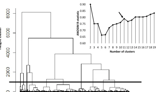
clusters grouping samples with very similar values). According to ANOSIM, the 195
Euclidean distance between the hierarchical classes is maximized with 11 clusters (see 196
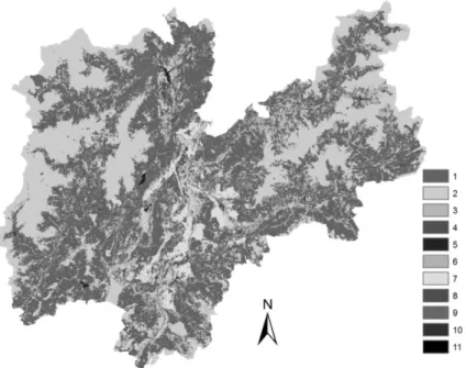
Figure 2). The map of ecosystem services clusters is in Figure 3. The explanation of 197
each bundle is detailed in Table 2, according to the spatial distribution and 198
types/values of ecosystem services. Information come from the analysis of the spatial 199
distribution of bundles and of the distribution of ecosystem services across bundles. 200
They are reported below. 201
Analysis of the spatial distribution of bundles
202
Shape analysis of bundles. Bundles are mapped over Trentino in Figure 3, which shows 203
that Bundles 1 covers the majority of the forested area, while Bundles 2 corresponds 204
to rocks and urban settlements, Bundles 3 is mainly present in the upper-eastern part, 205
while Bundles 7 occupies preferentially the central part. Fragmentation indices 206
highlight that Bundles 1 and Bundles 2 are the largest in area (occupying more than 207
40% of the region) and that the smallest are 8, 10 and 11 (occupying less than 0.1%). 208
fragmented one is Bundles 8, while the most compact ones are 1 and 9. For details see 210
Table 3. 211
Correlations with altitude. Bundles 2 shows a significant correlation ( = |0.4|) with 212
altitude (96% of its area lies above 2800 m a.s.l.) as well as and Bundles 11 (all the area 213
lies below 1000 m a.s.l.). Other bundles are homogeneously distributed across altitude 214
(Table 4, first row). 215
Correlations with catchments. Catchments are not significantly correlated to clusters. 216
However, small basins often lie in only one or two bundles (Table 4, second row). Only 217
the Adige catchment, that occupies the central part of Trentino, includes all bundles, 218
while Bundle 11 is only found in Adige catchment and in an eastern tributary. 219
Correlations with land use. Bundles 1 and 2 are correlated to land use (Table 4, third 220
row): Bundle 1 contains more than 90% of the whole forested area and Bundle 2 221
contains more than 90% of glaciers and bare rocks. Furthermore, forests contain more 222
than 90% of Bundles 3 and 11. 223
Analysis of the distribution of ecosystem services across bundles
224
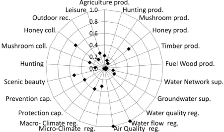
Analysis of the distribution of bundles across ecosystem services. The contribution of 225
the ecosystem services in each bundle is shown in 11 radar charts (Figure 7). For 226
example, Agriculture production is supplied in 5 bundles (2, 4, 7, 9 and 10); the 227
maximum provision is in Bundle 4, the minimum in Bundle 2. In all bundles, except 228
Bundle 2, there is at least one ecosystem service with maximum provision, and in all 229
bundles, except Bundle 3 and 8, there is at least one ecosystem service with minimum 230
(6,8), (1,3) and (9,10). The number of provisioning services per bundle ranges from 3 to 232
9 (out of 10); the number of regulating services ranges from 4 to 7 (out of 7); the 233
number of cultural services ranges from 4 to 7 (out of 8). 234
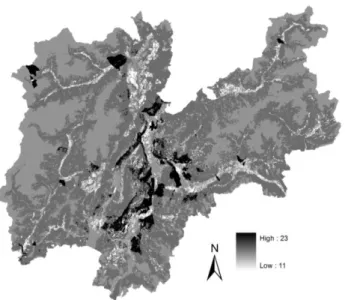
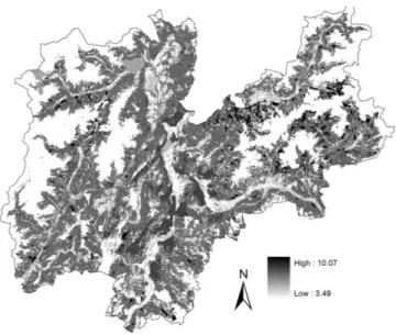
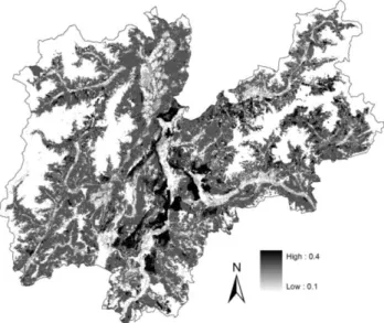
Aggregation patterns analysis. Aggregation patterns show that Bundle 9 has the 235
highest number of ecosystem services (i.e. 23 out of 25, cf. Figure 4 and Figure 5), 236
while Bundle 8 has the lowest one (i.e. 11 out of 25). Despite that, intensity of cluster 9 237
is lower than the intensity of Bundle 8 (6.75 against 8.6). Highest intensity and diversity 238
are in Bundle 3 (10.07 and 0.49 respectively, Figure 5 and Figure 6), while lowest 239
intensity and diversity are Bundle 2 (3.49 and 0.49 respectively). 240
4.2
Characterization of principal components
241Distribution of ecosystem services across principal components
242
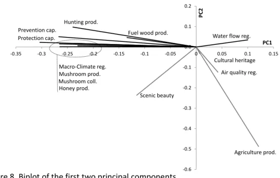
The loadings of Figure 8 show that PC1 is highly correlated to nine ecosystem services 243
(five provisioning, three regulating and one cultural service), while PC2 is highly 244
correlated to four ecosystem services (two regulating and two cultural services). PC1 245
and PC2 are therefore able to explain 13 ecosystem services (out of 25). 246
Distribution of principal components across bundles
247
Correlations between PC1 and bundles (Table 4) are significant for Bundles 1, 2, 3, 4 248
and 5, while correlations between PC2 and bundles are significant for Bundles 4, 5 and 249
Spatial distribution of principal components
251
The map in Figure 9 shows that low values of PC1 correspond to forest areas, while 252
high values to bare rocks, glaciers and urban settlements. Actually, the correlation of 253
PC1 with land use is high (|| = 0.7), while with altitude or catchments is not 254
significant. PC2 does not have any significant correlation. The analysis of correlations 255
with forest density showed that PC1 decreases for increasing values of forest density. 256
According to the characterization of principal components, two drivers of change 257
affect three bundles and seven ecosystem services in Trentino. Drivers are forest 258
management and land use management. The first driver affect bundle 1 (bundle of 259
most common ecosystem services in forests) and bundle 3 (bundle of forest areas of 260
high-intensity and high-diversity ecosystem services). Within the bundles, the 261
ecosystem service affected are Honey production, Mushroom production (and 262
collection), Fuel wood production and Macro-Climate regulation. The second driver 263
affect bundle 4 (bundle of agricultural areas of high-intensity ecosystem services) and 264
Agriculture production and Cultural heritage services. 265
5
Discussion
266To date only few studies have dealt with the definition of ecosystem services bundles 267
by means of analytical tools (e.g. Raudsepp-Hearne et al. 2009 and Plieninger et al. 268
2013) and even less studies have dealt with an analytical explanation of the ecosystem 269
services variability and of the drivers causing such variability (e.g. Raudsepp-Hearne et 270
theoretical framework of the ecosystem services bundles distribution and of drivers of 272
change, and these topics are still an open field of research (Anton et al. 2010). The 273
analyses proposed here allow the identification of the bundles to which each 274
ecosystem services belongs, and of the values of such ecosystem services in the 275
bundles. Moreover, they allow the identification of the factors that cause the main 276
variability of ecosystem services (i.e. land use and forest management) and the specific 277
ecosystem services on which they have great effect. 278
Principal components have been used here in order to avoid an a-priori selection of 279
indicators, and a statistical criterion (ANOSIM) has been used in order to optimize the 280
clustering. The characterization of the ecosystem services distribution across principal 281
components by means of loadings is a novel application in the definition of drivers of 282
change, as well as the computation of fragmentation indices to investigate the bundles 283
shape. The main merit of the proposed methodology is that of having organized the 284
analyses in a structured process where they are independent one from another. For 285
instance, a wider set of variables (not only altitude, land use distribution, etc.) may be 286
used to improve the knowledge about the spatial distribution of bundles. 287
In the present work, clusters of ecosystem services have been identified by means of a 288
limited number of principal components and bundles have been defined through a 289
narrow set of explanatory variables. However, the characterization of clusters is able 290
to provide a reasonable explanation for bundles. Trentino region is characterized by a 291
homogeneous distribution of ecosystem services, both in terms of type and value. In 292
to represent 98% of the territory. Four of them represent forest areas, corresponding 294
to 56% of the whole region. The fifth bundle represents poor-value ecosystem services 295
areas, covering about 40% of the territory, and consisting in urbanized areas, bare 296
rocks and other natural areas with low values of ecosystem services. On the other 297
hand, small bundles correspond to areas where the supply of a single service, or of a 298
narrow set of services, is very high with respect to other services. For instance, bundle 299
3 (that covers 7% of total forest areas) discriminates forests with high supply of fine-300
quality timber from the areas supplying the most common forest services. Such results 301
confirm what was found by Raudsepp-Hearne et al. (2009) and by Haines-Young et al. 302
(2012): the ecosystem services of a region group on a few number of bundles; this 303
number is smaller than the number of spatial units on which they are mapped 304
(municipalities in the case of Raudsepp-Hearne et al. 2009). In addition, bundles are 305
geographically clustered and little fragmentized across the territory. Finally, poor 306
ecosystem services areas group in one single bundle. 307
Drivers of change of ecosystem services have been investigated only for the first two 308
principal components, and by means of a narrow set of explanatory variables. It was 309
found that the supply of ecosystem services significantly changes across some forest 310
areas due to land use management activities (and especially due to the activities 311
involving forest loss). In particular, the highest supply variability is displayed by nine 312
typical forest ecosystem services, which are distributed over five bundles. This is in 313
accordance with findings of Steffan-Dewenter et al. (2007) and Haines-Young & 314
associated with the initial or the complete conversion of the forest to a different 316
ecosystem. Therefore, the study provides a solution to the problem of explaining the 317
factors that cause the main variability of ecosystem services. 318
According to Dale and Polasky (2007) ecosystem services are provided within process-319
related landscape units such as watersheds, specific habitats, or natural units (i.e. 320
intrinsic spatial units), and within such units, the ecosystem services values may be 321
heterogeneous. Anderson et al. (2009) pointed out that there are few studies on which 322
to base conclusions about the spatial relationships between habitats for different 323
ecosystem services and benefits for biodiversity, because such studies disregard spatial 324
heterogeneity. Syrbe and Walz (2012) stressed that this is a strong limitation for the 325
analyses that require a spatial representation of ecosystem services. The present study 326
attempts to consider intrinsic spatial heterogeneity for multiple ecosystem services 327
together. The cluster analysis showed that 25 ecosystem services are represented 328
together by 11 spatial units. It demonstrates that the intrinsic spatial heterogeneity of 329
sets of correlated ecosystem services (they are 11 bundles) is lower than the intrinsic 330
spatial heterogeneity of single ecosystem services (they were 20 spatial units of 331
representation for 25 ecosystem services). According to the results, bundles are also 332
different from the spatial units of single ecosystem services: the shape of bundles is 333
not only a combination of spatial units, but they are also dependent on the values of 334
single services in such units. Therefore, the number of clusters is lower than the spatial 335
A moderate degree of correlation was found between forest bundles and land use: the 337
only land use class that can be spatially recognized in bundles is that of forest. It 338
demonstrates that spatial units of land use are not sufficient to represent the spatial 339
heterogeneity of single ecosystem services, but one single spatial unit of land use (i.e. 340
forest) is sufficient to represent the spatial heterogeneity of multiple ecosystem 341
services. 342
6
Conclusions
343The method proposed in this study allows the mapping of a relevant number of 344
ecosystem services to be advanced, while accounting for the spatial heterogeneity of 345
the ecosystem services distribution and of their values. In particular, the study provides 346
a solution to the issue of defining the areas where sets of ecosystem services appear 347
together, i.e. bundles, and to the issue of explaining the factors that cause the main 348
variability of ecosystem services across the study region. 349
Management implications are to inform conservation efforts in the future, when there 350
is spatial heterogeneity of the ecosystem services provision. Considering that bundles 351
are sets of ecosystem services, their spatial representation depict areas that provide a 352
considerable amount of ecosystem services to humans. Hence, no matter their 353
biodiversity values, these areas could be given a protection status due to their 354
contribution to the wellbeing of the local population. 355
Future research could be devoted to the identification of areas offering an optimum 356
that additional social and ecological conditions may affect the ecosystem services 358
supply. For instance, demographic dynamics may influence the distribution of 359
ecosystem services supply, as well as be oriented by it. Understanding which factors 360
may have an actual influence requires the development of methods able to rank 361
ecosystem services and to explain the relations between these services and the social 362
References
364
1. Anderson BJ, Armsworth PR, Eigenbrod F, Thomas CD, Gillings S, Heinemeyer H, 365
Roy DB, Gaston KJ. 2009. Spatial covariance between biodiversity and other 366
ecosystem service priorities. Journal of Applied Ecology. 46:888–896. 367
2. Anton C, Young J, Harrison PA, Musche M, Bela G, Feld CK, Harrington C, Haslett 368
JR, Pataki G, Rounsevell MDA, Skourtos M, Sousa JP, Sykes MT, Tinch R, 369
Vandewalle M, Watt A, Settele J. 2010. Research needs for incorporating the 370
ecosystem service approach into EU biodiversity conservation policy. 371
Biodiversity Conservation. 19:2979–2994. 372
3. Bennet EM, Peterson GD, Gordon LJ. 2009. Understanding relationships among 373
multiple ecosystem services. Ecology Letters. 12:1-11. 374
4. Carpenter SR, DeFries R, Dietz T, Mooney HA, Polasky S, Reid WV, Scholes RJ. 375
2006. Millennium ecosystem assessment: research needs. Science. 314: 527-376
258. 377
5. Clarke KR. 1993. Non-parametric multivariate analysis of changes in community 378
structure. Australian Journal of Ecology. 18:117-143. 379
6. Dale VH, Polasky S. 2007. Measures of the effects of agricultural practices on 380
ecosystem services. Ecological Economics. 64(2): 286–296. 381
7. Daily GC, Matson PA. 2008. Ecosystem services: from theory to 382
implementation. PNAS. 105(28):9455-9456. 383
8. Ferrari M. 2014. Spatial assessment of multiple ecosystem services in an Alpine 384
9. Ferrari M, Geneletti D, Cayuela L, Benayas JM. Submitted. Identifying key 386
indicators to assess multiple ecosystem services and their interactions at 387
regional scale. Environmental Management. 388
10. Haines-Young R, Potschin M. 2010a. Proposal for a Common International 389
Classification of Ecosystem Goods and Services (CICES) for Integrated 390
Environmental and Economic Accounting. Report to the EEA. 391
11. Haines-Young R, Potschin, M, 2010b. The links between biodiversity, ecosystem 392
services and human well-being. Ecosystem Ecology: A New Synthesis, 393
Cambridge University Press. 394
12. Haines-Young R, Potschin M, Kienast F. 2012. Indicators of ecosystem service 395
potential at European scales. Ecological Indicators. 21:39–53. 396
13. Hodder KH, Newton CN, Elena Cantarello E,Perrella L. 2014. Does landscape-397
scale conservation management enhance the provision of ecosystem services? 398
1(10):71-83. 399
14. Kaufman L, Rousseeuw PJ. 1990. Finding groups in data: an introduction to 400
cluster analysis. Wiley editor. 401
15. Maes, J. et al. 2012. Mapping ecosystem services for policy support and 402
decision making in the European Union. Ecosystem services, Volume 1, pp. 31-403
39. 404
16. Maes J, Egoh B, Willemen L, Liquet C, Vihervaara P, Schägner JP, Grizzetti B, 405
2012a. Mapping ecosystem services for policy support and decision making in 407
the European Union. Ecosystem Services. 1:31-39. 408
17. Maes J, Paracchini ML, Zulian G, Dunbar MB, Alkemade R. 2012b. Synergies and 409
trade-offs between ecosystem service supply, biodiversity, and habitat 410
conservation status in Europe. Biological Conservation. 155:1–12. 411
18. Maes J, Paracchini ML, Zulian G, 2011a. An European assessment of ecosystem 412
services. Towards an atlas of ecosystem services. ISPRA: Partnership for 413
European Environmental Research. 414
19. Maes J, Braat L, Jax K, Hutchins M, Furman E, Termansen M, Luque S, Paracchini 415
ML, Chauvin C, Williams R, Volk M, Lautenbach S, Kopperoinen L, Schelhaas MJ, 416
Weinert J, Goossen M, Dumont E, Strauch M, Görg C, Dormann C, Katwinkel M, 417
Zulian G, Varjopuro R, Ratamäki O, Hauck J, Forsius M, Hengeveld G, Perez-418
Soba M, Bouraoui F, Scholz M, Schulz-Zunkel C, Lepistö A, Polishchuk Y, Bidoglio 419
G. 2011b. A spatial assessment of ecosystem services in Europe: methods, case 420
studies and policy analysis—phase 1. PEER Report no. 3. Ispra: Partnership for 421
European Environmental Research. 422
20. Martínez-Harmsa MJ, Balvanera P. 2012. Methods for mapping ecosystem 423
service supply: a review. International Journal of Biodiversity Science, 424
Ecosystem Services & Management. 8(1-2):17-25. 425
21. Maskel LC, Crowe A, Dunbar MJ, Emmett B, Henrys P, Keith AM, Norton LR, 426
Scholefield P, Clark DB, Simpson IC, Smart SM. 2013. Exploring the ecological 427
22. Millennium Ecosystem Assessment (MA). 2005. Ecosystems and human well-429
being: synthesis. Washington (DC): Island Press 430
23. Naidoo R, Balmford A, Costanza R, Fisher B, Green RE, Lehner B, Malcolm TR, 431
Ricketts TH. 2008. Global mapping of ecosystem services and conservation 432
priorities. PNAS. 105:9495-9500. 433
24. Pearson K. 1901. On Lines and Planes of Closest Fit to Systems of Points in 434
Space. Philosophical Magazine, 2(11):559-572. 435
25. Plieninger T, Fijks S, Oteros-Rozas E, Bieling C. 2013. Assessing, mapping and 436
quantifying cultural ecosystem services at community level. Land Use Policy. 437
33:118-129. 438
26. Qiu J, Turner MG. 2013. Spatial interactions among ecosystem services in an 439
urbanizing agricultural watershed. PNAS 11(29):12149-12154. 440
27. Raudsepp-Hearne C, Peterson GD, Bennett EM. 2009. Ecosystem service 441
bundles for analyzing tradeoffs in diverse landscapes. PNAS Early Edition. pp:1-442
6. 443
28. Uta Schirpke U, Georg Leitinger G, Erich Tasser E, Markus Schermer M, Melanie 444
Steinbacherc M, Tappeiner U. 2013. Multiple ecosystem services of a changing 445
Alpine landscape: past, present and future. 9(2):123-135. 446
29. Syrbe RU, Walz U. 2012. Spatial indicators for the assessment of ecosystem 447
services: Providing, benefiting and connecting areas and landscape metrics. 448
30. Shannon, CE. 1948. A mathematical theory of communication. The Bell System 450
Technical Journal, 27: 379–423 and 623–656. 451
31. Schulz JJ, Cayuela L, Rey-Benayas JM., Schroder B. 2011. Factors influencing 452
vegetation cover change in Mediterranean Central Chile (1975-2008). Applied 453
Vegetation science. 14:571-582. 454
32. Steffan-Dewenter I, Kessler M, Barkmann J, Bos MM, Buchori D. 2007. 455
Tradeoffs between income, biodiversity, and ecosystem functioning during 456
tropical rainforest conversion and agroforestry intensification. PNAS. 457
104:4973–4978. 458
33. van Oudenhoven APE, de Groot RS. 2013. Trade-offs and synergies between 459
biodiversity conservation, land use change and ecosystem services. 460
International Journal of Biodiversity Science, Ecosystem Services & 461
Management. 9(2): 87-89. 462
34. van Oudenhoven APE, Petz K, Alkemade R, de Groot RS. 2012. Framework for 463
systematic indicator selection to assess effects of land management on 464
ecosystem services. Ecological Indicators. 21:110–122. 465
35. Willemen L, Verburg PH, Hein L, van Mensvoort MEF. 2008. Spatial 466
Characterization of landscape functions, Landscape and Urban Planning 88:34-467
59
TABLES
1
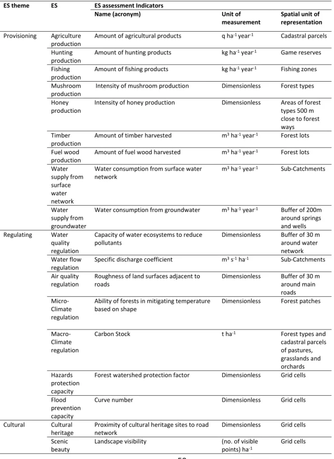
Table 1. 24 ecosystem services (ES, 2nd column) are grouped in three themes (1st column) and 2
assessed by 24 indicators. Indicators are mapped over different spatial units (4th column). 3
ES theme ES ES assessment Indicators
Name (acronym) Unit of
measurement
Spatial unit of representation
Provisioning Agriculture
production
Amount of agricultural products q ha-1 year-1 Cadastral parcels
Hunting production
Amount of hunting products kg ha-1 year-1 Game reserves
Fishing production
Amount of fishing products kg ha-1 year-1 Fishing zones
Mushroom production
Intensity of mushroom production Dimensionless Forest types
Honey production
Intensity of honey production Dimensionless Areas of forest
types 500 m close to forest ways
Timber production
Amount of timber harvested m3 ha-1 year-1 Forest lots
Fuel wood production
Amount of fuel wood harvested m3 ha-1 year-1 Forest lots
Water supply from surface water network
Water consumption from surface water network
m3 ha-1 year-1 Sub-Catchments
Water supply from groundwater
Water consumption from groundwater m3 ha-1 year-1 Buffer of 200m
around springs and wells
Regulating Water
quality regulation
Capacity of water ecosystems to reduce pollutants
Dimensionless Buffer of 30 m
around water network Water flow
regulation
Specific discharge coefficient m3 s-1 ha-1 Sub-Catchments
Air quality regulation
Roughness of land surfaces adjacent to roads
Dimensionless Buffer of 30 m
around main roads
Micro-Climate regulation
Ability of forests in mitigating temperature based on shape
Dimensionless Forest patches
Macro-Climate regulation
Carbon Stock t ha-1 Forest types and
cadastral parcels of pastures, grasslands and orchards Hazards protection capacity
Forest watershed protection factor Dimensionless Grid cells
Flood prevention capacity
Curve number Dimensionless Grid cells
Cultural Cultural
heritage
Proximity of cultural heritage sites to road network
Dimensionless Grid cells
Scenic beauty
Landscape visibility (no. of visible
points) ha-1
Grid cells
60
Hunting Density of hunters (no. of hunters)
ha-1 year-1
Game reserves
Fishing Fishing intensity (no. of fishing
activities) ha-1
year-1
Fishing zones
Mushroom collection
Availability of mushrooms of good quality Dimensionless Forest types
Honey collection
Availability of honey of good quality Dimensionless Areas of forest
types 150 m close to forest ways
Outdoor recreation
Intensity of sporting activities (no. of sport
activities) ha-1
Patches of lakes, forest roads and ski slopes
Leisure Density of recreational activities Dimensionless Patches of lakes
and forest types
61
Table 2. 11 bundles are the sets of spatially correlated ecosystem services in Trentino. They are 5
explained according to the spatial distribution and to the number, types and values of ecosystem 6
services. 7
Bundles of Spatial distribution of bundles Number, types and values of ecosystem services in the bundles
1
Most common ecosystem services in forests
The bundle corresponds to 90% of forest areas of Trentino up to 2800 m a.s.l.. It is composed
of few, large and little
fragmented patches.
18 ecosystem services are supplied: four provisioning, seven regulating and seven cultural. They are typically of forest ecosystems. The provision is maximum for Honey production and Micro-Climate regulation services.
2
Low-intensity and
low-diversity ecosystem
services
The bundle includes 90% of the areas above 2800m a.s.l., which are essentially glaciers and bare rocks. It is composed of few, large and little fragmented patches.
The bundle covers the areas where the supply of ecosystem services is the lowest in terms of intensity and diversity. 17 services are supplied: three provisioning, seven regulating and seven cultural. With respect to other bundles, the supply is not maximum for any ecosystem service. It is minimum for five ecosystem services: Agriculture production, Micro-Climate regulation, Mushroom and Honey collection and Leisure.
3
High-intensity and
high-diversity ecosystem
services in forests
The bundle is covered for 90% by forest areas, corresponding to the forest areas of Val di Fiemme, where the use of forest services, like timber production, is very high.
18 services are supplied: five provisioning, six regulating and seven cultural. The supply is maximum for six services: Hunting, Mushroom, Honey and Timber production, Micro-Climate regulation and Hunting activity. With respect to other bundles, the supply of forest ecosystem services is the highest in terms of intensity and diversity.
4
High-intensity
ecosystem services in agriculture areas
The bundle covers the
agricultural areas up to 1000m a.s.l..
13 ecosystem services are supplied: three provisioning, six regulating and four cultural. With respect to other bundles, the supply of Agriculture production and Cultural heritage is maximum, while the supply of water regulation services (i.e. Water quality and Water flow regulation) is minimum.
5
High-intensity recreation services in forests and over water network
This bundle covers forest areas and fishing zones up to 2800m a.s.l..
17 ecosystem services are supplied: four provisioning, six regulating and seven cultural. With respect to other bundles, he supply of Leisure and Outdoor activities is maximum.
6
High capacity in water regulation
It is a small bundle composed
of fragmented patches,
homogeneously distributed
over catchments up to 2800 m a.s.l.. It is typical of minor tributaries in the lateral valleys.
13 ecosystem services are supplied: three provisioning, five regulating and five cultural. The supply is maximum for two services: Water quality regulation and Flood prevention capacity.
7
High-intensity human
activities in
semi-urbanized areas
The bundle covers the central areas of the region, up to 1000m a.s.l.,
23 ecosystem services are supplied: eight provisioning, seven regulating and seven cultural. The supply is maximum for Hunting and Scenic beauty.
8
Lowest number of
ecosystem services and high-intensity values
It is a small bundle composed
of fragmented patches,
homogeneously distributed
over catchments up to 1000m a.s.l..
11 ecosystem services are supplied: three provisioning, four regulating and four cultural. With respect to other bundles, it is the less rich of ecosystem services. The supply is maximum for six ecosystem services: Hunting production, Fishing production and activity, Water supply from groundwater, Hazard protection capacity and Outdoor recreation.
9
Highest number of
ecosystem services and low-intensity values
The bundle is composed of few, large and little fragmented patches. It is homogeneously
distributed over altitude,
catchments and it covers all land uses.
23 services ecosystem services are supplied: 10 provisioning, seven regulating and seven cultural. With respect to other bundles, it is the richest of ecosystem services. The supply is not maximum for any service. Instead. It is minimum for: Water supply from surface water network, Cultural heritage and Outdoor recreation.
10
High-intensity regulating services
The bundle is homogeneously distributed over altitude up to 1000m a.s.l..
21 ecosystem services are supplied: eight provisioning, seven regulating and six cultural. The supply is maximum for two regulating services: Water flow regulation and Air quality regulation.
62
Ecosystem services in low-elevation forests
only 3 patches. All areas are below 1000m a.s.l. and they correspond to forests for more than 90%.
63 Table 3. Shape analysis of bundles
8
Bundles Area
[%]
Number of patches [No.]
Min patch area [ha]
Max patch area [ha]
Mean patch area [ha]
Fragmentation index
[Dimensionless]
1 45.773 6767 1 96555 41.6 0.0
2 40.133 17362 1 54225 14.2 0.1
3 3.465 2642 1 653 8.1 0.1
4 4.901 7882 1 935 3.8 0.3
5 0.599 1655 1 326 2.2 0.4
6 0.166 530 1 85 1.9 0.5
7 4.106 1831 1 4546 13.8 0.1
8 0.016 69 1 6 1 0.7
9 0.816 20 1 2030 250.6 0.0
10 0.024 8 1 69 18.75 0.1
11 0.002 3 1 10 4 0.3
64
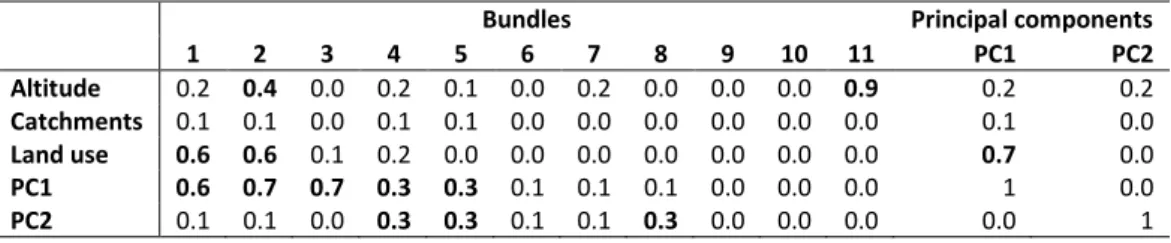
Table 4. Spearman correlation coefficients of bundles and principal components with altitude, 11
catchments and land use. We consider significant correlations (bolded text) when correlation 12
coefficients are greater than or equal to 0.3. 13
Bundles Principal components
1 2 3 4 5 6 7 8 9 10 11 PC1 PC2
Altitude 0.2 0.4 0.0 0.2 0.1 0.0 0.2 0.0 0.0 0.0 0.9 0.2 0.2
Catchments 0.1 0.1 0.0 0.1 0.1 0.0 0.0 0.0 0.0 0.0 0.0 0.1 0.0
Land use 0.6 0.6 0.1 0.2 0.0 0.0 0.0 0.0 0.0 0.0 0.0 0.7 0.0
PC1 0.6 0.7 0.7 0.3 0.3 0.1 0.1 0.1 0.0 0.0 0.0 1 0.0
PC2 0.1 0.1 0.0 0.3 0.3 0.1 0.1 0.3 0.0 0.0 0.0 0.0 1
14
59
FIGURES
1
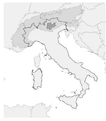
2
Figure 1. Trentino region within the Alps in Italy 3
60 5
6
7
Figure 2. In clustering the most significant difference between the groups is realized for 11 clusters 8
(local maximum of the ANOSIM, arrow), which corresponds to about 1000 of height in the 9
dendogram (horizontal line). 10
11
Euclidean distance between statistical units of principal components
H
e
ig
h
t c
lu
ste
r
0.60 0.65 0.70 0.75 0.80 0.85 0.90
2 3 4 5 6 7 8 9 10 11 12 13 14 15 16 17 18 19
AN
OSIM
R
-s
ta
tis
tic
61 12
Figure 3. Map of 11 clusters, i.e. bundles of ecosystem services 13
62 15
16
Figure 4. Richness index 17
63 19
20
Figure 5. Intensity index 21
64 23
24
25
Figure 6. Diversity index 26
60 Cluster 1 0.0 0.2 0.4 0.6 0.8 1.0 Mushroom prod. Honey prod. Timber prod.
Fuel Wood prod.
Water quality reg.
Water flow reg.
Air Quality reg.
Micro-Climate reg. Macro- Climate reg. Protection cap. Prevention cap. Cultural heritage Scenic beauty Hunting Mushroom coll. Honey coll. Outdoor rec. Leisure Cluster 2 0.00 0.20 0.40 0.60 0.80 1.00 Agriculture prod. Honey prod.
Water quality reg.
Water flow reg.
Air Quality reg.
Micro-Climate reg. Macro-Climate reg. Protection cap. Prevention cap. Cultural heritage Scenic beauty Hunting Mushroom coll. Honey coll. Outdoor rec. Leisure Cluster 3 0.0 0.2 0.4 0.6 0.8 1.0 Hunting prod. Mushroom prod. Honey prod. Timber prod.
Fuel Wood prod.
Water quality reg.
Water flow reg.
Air Quality reg. Micro-Climate reg. Macro- Climate reg.
Protection cap. Cultural heritage Scenic beauty Hunting Mushroom coll. Honey coll. Outdoor rec. Cluster 4 0.0 0.2 0.4 0.6 0.8 1.0 Agriculture prod. Hunting prod. Groundwater sup.
Water quality reg.
Water flow reg.
Air Quality reg.
61 Cluster 5 0.0 0.2 0.4 0.6 0.8 1.0 Hunting prod. Fishing prod. Honey prod. Groundwater sup.
Water quality reg.
Water flow reg.
Air Quality reg.
Macro- Climate reg. Protection cap. Prevention cap. Cultural heritage Scenic beauty Fishing Mushroom coll. Honey coll. Outdoor rec. Leisure Cluster 6 0.0 0.2 0.4 0.6 0.8 1.0 Hunting prod. Fishing prod. Groundwater sup.
Water quality reg.
Water flow reg.
Air Quality reg.
Protection cap. Prevention cap. Scenic beauty Hunting Fishing Outdoor rec. Leisure Cluster 7 0.0 0.2 0.4 0.6 0.8 1.0 Agriculture prod. Hunting prod. Mushroom prod. Honey prod.
Inorganic matter ext.
Timber prod.
Fuel Wood prod.
Groundwater sup.
Water quality reg. Water flow reg. Air Quality reg. Micro-Climate reg.
Macro- Climate reg. Protection cap. Prevention cap. Cultural heritage Scenic beauty Hunting Mushroom coll. Honey coll.
Outdoor rec.Leisure
Cluster 8 0.0 0.2 0.4 0.6 0.8 1.0 Hunting prod. Fishing prod. Groundwater sup.
Water quality reg.
Water flow reg.
62 0.00 0.20 0.40 0.60 0.80 1.00 Agriculture prod. Hunting prod. Mushroom prod. Honey prod. Timber prod.
Fuel Wood prod.
Water Network …
Ground water sup.
Water quality reg. Water flow reg. Air Quality reg. Micro-Climate reg. Macro-Climate reg. Protection cap. Prevention cap. Cultural heritage Scenic beauty Hunting Mushroom coll. Honey coll.
Outdoor rec.Leisure
Cluster 9 Cluster 10 0.0 0.2 0.4 0.6 0.8 1.0 Agriculture prod. Hunting prod. Mushroom prod. Honey prod. Timber prod.
Fuel Wood prod.
Water Network sup.
Groundwater sup.
Water quality reg. Water flow reg. Air Quality reg. Micro-Climate reg.
Macro- Climate reg. Protection cap. Prevention cap. Scenic beauty Hunting Mushroom coll. Honey coll. Outdoor rec. Leisure Cluster 11 0.0 0.2 0.4 0.6 0.8 1.0 Hunting prod. Mushroom prod. Honey prod. Timber prod.
Fuel Wood prod.
Water Network sup.
Groundwater sup.
Air Quality reg. Micro-Climate reg.
Macro- Climate reg. Prevention cap. Scenic beauty Hunting Mushroom coll. Honey coll. Leisure
Figure 7. Contribution of the ecosystem services to 11 bundles. Each ecosystem service is represented by one indicator, whose values
63
Agriculture prod. Hunting prod.
Honey prod. Mushroom prod.
Fuel wood prod. Water flow reg.
Air quality reg. Macro-Climate reg.
Protection cap. Prevention cap.
Cultural heritage
Scenic beauty Mushroom coll.
-0.6 -0.5 -0.4 -0.3 -0.2 -0.1 0.0 0.1 0.2
-0.35 -0.3 -0.25 -0.2 -0.15 -0.1 -0.05 0 0.05 0.1 0.15
PC2
PC1
1
Figure 8. Biplot of the first two principal components 2
64 4
5
Figure 9. Distribution of PC1 scores among forest areas and other areas. 56% of 6
Trentino is forest (the grey area in the picture); lowest values of PC1 are in forest 7