Hybrid diffuse optics for monitoring of tissue hemodynamics with applications in oncology

(1)

ICFO · THE INSTITUTE OF PHOTONIC SCIENCES

AV. CARL FRIEDRICH GAUSS, 3 · CASTELLDEFELS · BARCELONA &

UPC · UNIVERSITAT POLITÈCNICA DE CATALUNYA CAMPUS NORD · BARCELONA

PARISA FARZAM

Advisor:

Turgut Durduran

PhD Thesis 2014

P

ARISA F

ARZAM

HYBRID DIFFUSE OPTICS FOR MONITORING

OF TISSUE HEMODYNAMICS WITH APPLICA

TIONS IN ONCOLOGY

Hybrid diffuse optics for monitoring

of tissue hemodynamics with

applications in oncology

D O C T O R A L T H E S I S I N P H O T O N I C S

I C F O B A R C E L O N A 2 0 1 4

(2)

(3)

Doctor of Philosophy in Photonics

Institute of Photonic Sciences (ICFO)

Hybrid diffuse optics for

monitoring of tissue hemodynamics

with applications in oncology

by

_{Parisa Farzam}

Ph.D. Dissertation

(4)

(5)

(6)

(7)

Declaration

I hereby declare that except where specific reference is made to the work of others, the contents of this dissertation are original 1 and have not

been submitted in whole or in part for consideration for any other degree or qualification in this, or any other university.

Parisa Farzam July 2014

1Two photos in the cover page are adopted from from:

http://www.wikihow.com/Draw-a-Cartoon-Skeleton and

(8)

(9)

Acknowledgements

It is a great pleasure for me to acknowledge all the people who have supported me with their love and helped me to get to this point. Turgut is definitely on top of my list. I met Prof. Turgut Durduran in one of his amazing lectures. After his talk, I was absolutely sure that I want to peruse my academic career in his lab. I was lucky enough to be his first PhD student at ICFO and this gave me the invaluable opportunity to have his presence in the lab, long discussions, and deep education. Turgut is a brilliant advisor whose talent, creativity, critical thinking, and hardworking make him a special person. He aimed to make an independent researcher out of me and now I feel confident to find new problems and step forward to solve them on my own. He was not only a wonderful advisor, but he was also a great friend who has helped me in all my difficulties. I have no words to show my respect to him.

My research was not possible without the support of excellent clinical collaborators. I consider it an honor to work with Dr. Oriol Casanovas, Dr. Alvaro Urbano, Dr. Angels Sierra, and Dr. Tiziano Binzoni. Al-though I won’t be able to list all our collaborators, I owe my deepest gratitude to all of them.

(10)

Dr. Regine Choe who has been always welcoming to my questions and discussions.

I share the credit of my work with all my colleagues and my good friends in medical optics group, including Peyman Zirak, Johannes Jo-hanson, Hari Varma, Igor Blanco, Claudia Valdes, Claus Lindner, Taisuke Minagawa, Mehmet Suzen, Alexia Giannoula, Udo Weigel, Juan Aguirre, Anna Kristoffersen, Francisco Remiro, Miguel Mireles, Jordi Morales Dalmau, Clara Gregori, Tanja Dragojevic, Marco Pagliazzi, Martina Giovannella, Victor Chamizo and many more. You made these years full of good memories. I miss all 32 of you. Are you really counting? Then include Maria please! Beside the medical optics group, I am deeply grateful to all ICFOnians specially Prof. Lluis Torner whose remarkable management made ICFO a fabulous center, Prof. Majid Ebrahim-Zadeh my respected advisor in master project who helped me a lot from my very first day in Barcelona, and Prof. David Artigas who was always kindly there to help me when I was lost and confused. I am thankful of ICFO’s human resources (Anne, Laia, Mery, Manuela and Cristina), electronic and mechanical workshop and all my friends at ICFO.

During my PhD, I lost my beloved grandma without having the chance to say goodbye to her. She was my angle who treated me with pure love and good tea. I share my graduation happiness with her memory and with my lovely friends, cousins, aunts and uncles. I do not list your names here but I am grateful to have all of you in my life.

My heartfelt appreciation goes to my beloved father (Jafar), my amazing mother (Soori), and my awesome brother (Arash). You three are the light of my life. I can not think of a better place to grow rather than a house with you.

(11)

Abstract

Hybrid diffuse optics for

monitoring of tissue hemodynamics

with applications in oncology

Parisa Farzam

Noninvasive measurement of hemodynamics at the microvascular level may have a great impact on oncology in clinics for diagnosis, ther-apy planning and monitoring, and, in preclinical studies. To this end, diffuse optics is a strong candidate for noninvasive, repeated, deep tissue monitoring.

In this multi-disciplinary, translational work, I have constructed and deployed hybrid devices which are the combination of two qualitatively different methods, near infrared diffuse optical spectroscopy (NIRS) and diffuse correlation spectroscopy (DCS), for simultaneous measurement of microvascular total hemoglobin concentration, blood oxygen satura-tion and blood flow.

(12)

In two in vivo studies in human volunteers, I have developed

pro-tocols and probes to demonstrate the feasibility of noninvasive diffuse optical spectroscopy to investigate the pathophysiology of bone. First study was study on the physiology of the patella microvasculature, the other introduced the manubrium as a site that is rich in red bone mar-row and accessible to diffuse optics as a potential window to monitor the progression of hematological malignancies.

(13)

Resumen

Óptica difusa híbrida para la

monitorización de la hemodinámica de los

tejidos con aplicaciones en oncología

Parisa Farzam

La medición no invasiva de la hemodinámica a nivel microvascular puede alcanzar un gran impacto en oncología: en las clínicas para el di-agnóstico, la planeación y monitorización de las terapias, y en estudios preclínicos. La óptica difusa es una fuerte candidata para la monitor-ización no invasiva y repetida del tejido profundo.

En este trabajo multidisciplinario y traslacional, construí e imple-menté dispositivos híbridos que son la combinación de dos métodos cualitativamente diferentes: espectroscopía infrarroja de óptica difusa -near infrared diffuse optical spectroscopy (NIRS)- y espectroscopía de correlación de luz difusa -diffuse correlation spectroscopy (DCS)-. Es-tos híbridos permiten la medición simultánea de la concentración de hemoglobina total en sangre, la saturación de oxígeno y el flujo sanguí-neo.

(14)

tempranos, lo cual proporciona información valiosa para un mejor en-tendimiento del mecanismo de resistencia de los tumores a las terapias antiangiogénicas.

En dos estudiosin vivorealizados en pacientes voluntarios, desarrollé

protocolos y sondas para demostrar la viabilidad de la espectroscopía de óptica difusa no invasiva en el estudio de la patofisiología ósea. El primer estudio se concentró en la fisiología microvascular de la rótula y en el otro se muestra que el manubrio, hueso rico en médula ósea roja, es un sitio accesible para la óptica difusa, y se presenta como una ventana para monitorizar la progresión de enfermedades hematológicas malignas.

(15)

List of figures

1.1 Physiological window. . . 2 1.2 Light experiences multiple scattering in tissues. . . 3 1.3 The spectrum of hypoxic tumor in comparison to healthy

tissue. . . 4

2.1 Three types of light sources: continuous wave, intensity modulated, and pulsed. . . 11 2.2 The dependency of diffuse wave density wavevector on

modulation frequency. . . 13 2.3 The phase shift and ln(Aρ) as a function of optode

dis-tances in an infinite turbid medium. . . 14 2.4 The dependency of DPDW wavelength (λDP DW) on

op-tical properties of the medium and modulation frequency. 15 2.5 Dependency of amplitude on medium and source. . . 17 2.6 Dependency of phase on medium and source . . . 18 2.7 Extrapolated zero boundary to approximate fluence rate. 19 2.8 The phase shift and ln(Aρ) as a function of optode

dis-tances in semi-infinite boundary condition. . . 21 2.9 Light propagation in tissues. . . 22 2.10 The probability of detecting photons from different depths. 23 2.11 Effect of different parameters on the shape of field

(20)

3.1 Optical probe on the murine tumor. . . 34

3.2 The schematic of broadband NIRS device. . . 36

3.3 The schematic of diffuse correlation spectroscopy device. 38 3.4 The schematic of a semicircle probe with uniform distri-bution of 8 detectors and simulated intensity from each detector. . . 39

3.5 The schematic of desired self-calibrating probe. . . 40

3.6 Simulated detected intensity of 8 detector positions sat-isfying all the desired constraints in the probe design. . . 41

3.7 The schematic of hand-held NIRS-DCS probe. . . 42

3.8 A picture of probe tip. . . 43

3.9 The quantum efficiency spectrum of the CCD. . . 46

3.10 The effect of calibration on the measured values. . . 48

3.11 The effect of calibration on the quality of fitting. . . 49

3.12 Results of phantom measurement with broadband NIRS. 51 3.13 The procedure of cuff occlusion on the mouse’s thigh. . . 51

3.14 Hemodynamics changes induced by mouse cuff occlusion. 52 4.1 Newly developed tumorgraft mouse model to study an-tiangiogenic therapies. . . 58

4.2 Physiological characterization of the RCC tumor in com-parison with a control muscle. . . 60

4.3 Correlation between DOS and DCS values. . . 61

4.4 Measured blood flow over time shows that all the treated animals have an initial drop in the blood flow. . . 63

4.5 Tumor growth in time. . . 64

4.6 The extracted tumor weight. . . 65

4.7 Degree of vascularization in the extracted tumor. . . 66

(21)

List of figures xix

4.9 Correlation between initial change in blood flow and the

blood vessel density. . . 67

4.10 Correlation between initial change in blood flow and time-to-progress in treated tumors. . . 68

5.1 The protocol of measurement on the manubrium. . . 78

5.2 The distribution of the measured parameters. . . 83

5.3 Changes of physiological parameters over 4 locations. . . 85

5.4 Correlation between the measured parameters. . . 85

5.5 Correlation between BMI and skinfold values. . . 86

5.6 Correlation of the skinfold values and hemodynamics. . . 87

5.7 Correlation of the BMI and measured hemodynamics. . . 87

5.8 Distribution of the measured parameters by gender . . . 88

5.9 Correlation of age and measured hemodynamics. . . 89

5.10 measurement repeatability on different locations. . . 95

5.11 The effect of probe pressure on the measurement . . . 96

6.1 Probe design and its placement on the knee. . . 105

6.2 Measurement protocol on the patella. . . 106

6.3 Calibration effect and fitting quality in simulation. . . 110

6.4 An example of fitting quality. . . 115

6.5 Patella hemodynamics during cuff-occlusion. . . 117

6.6 An example of amplitude and phase pulsation. . . 118

6.7 The pulsation of absorption and scattering coefficients. . 120

6.8 The pulsation of measured physiological parameters. . . . 121

7.1 The systematic error in measured blood flow. . . 132

7.2 The effect of µs′ error on BFI calculation. . . 133

7.3 The effect of µa error on BFI calculation. . . 134

7.4 Similarity of autocorrelation curves in different media. . . 136

(22)

7.6 The error in fitted BFI by MD-DCS comparing to other methods in noise-free data. . . 143 7.7 The fitted µa, µs′, and BFI by MD-DCS for noise-added

data in small optode distances. . . 144 7.8 The error in fitted BFI with MD-DCS in noise-added

sim-ulated data in small optode distances. . . 145 7.9 The fitted µa, µs′, and BFI by MD-DCS for noise-added

data in intermediate optode distances. . . 146 7.10 The error in fitted BFI with MD-DCS in noise-added

sim-ulated data in intermediate optode distances. . . 147 7.11 The fitted µa, µs′, and BFI by MD-DCS for noise-added

data in large optode distances. . . 148 7.12 The error in fitted BFI with MD-DCS in noise-added

sim-ulated data in large optode distances. . . 149 7.13 MD-DCS measurements on liquid phantom. . . 150 7.14 MD-DCS measurements on mouse tumor. . . 151

(23)

List of tables

5.1 Vital records of the recruited subjects. . . 76 5.2 Physical characteristics of the recruited subjects. . . 77 5.3 The measured physiological parameters. . . 82 5.4 The fitted value for the first location and the slope. . . . 84 5.5 Effect of assuming different concentrations of lipid and

bone mineral on measured values. . . 93

6.1 The measured optical and physiological values. . . 116 6.2 µa and µs′ changes during one cardiac cycle. . . 119

C.1 Absorption coefficient of the manubrium. . . 203 C.2 Reduced scattering coefficient of the manubrium. . . 205 C.3 Physiological parameters of the manubrium. . . 206

D.1 µa values of the patella during rest. . . 209

D.2 µs′ values of the patella during rest. . . 210

D.3 Measured physiological parameters during rest. . . 211 D.4 µa values of the patella at the end of cuff occlusion. . . . 211

(24)

(25)

Nomenclature

α fraction of dynamic photon scattering events in medium

ci concentration of the ith chromophore

D photon diffusion coefficient, D=ν/3(µa+µs′)

Db Brownian diffusion coefficient

ϵ extinction coefficient

g scattering anisotropy factor

G0 homogeneous Green’s function solution of diffusion equation

G1 electric field temporal autocorrelation function,

G1(ρ, τ, t) =< E∗(ρ, t)E(ρ, t+τ)>

G2 intensity autocorrelation function,

G2(ρ, τ, t) =< I(ρ, t)I(ρ, t+τ)>

g1 normalized electric field temporal autocorrelation function,

g1(ρ, τ, t) =G1(ρ, τ, t)/ < E∗(ρ, t)E(ρ, t)>

g2 normalized intensity autocorrelation function,

g2(ρ, τ, t) =G2(ρ, τ, t)/ < I(ρ, t)I(ρ, t)>

(26)

ltr transport mean-free path, ltr ≈1/µs′

λ wavelength of light (nm)

λDP DW wavelength of diffuse photon wave density (nm)

µa absorption coefficient

µs scattering coefficient

µs′ reduced scattering coefficient, µs′ =µs(1−g)

ν speed of light in tissue

⟨∆r2(_τ)_⟩ mean-square displacement in time _τ of the scattering

par-ticles (e.g., red blood cells)

Φ(ρ, t) photon-fluence rate at positionρ and time t

ρ distance between source and detector

τ delay time

U(ρ) photon-fluence rate; expressed in the frequency domain,

Φ(ρ, t) = U(ρ)e−iwt

ω source modulation frequency

Abbreviations

BFI blood flow index estimated by DCS (i.e., αDb)

BMI body mass index

CCD charge-coupled device

CT computed tomography

(27)

Nomenclature xxv

DCS diffuse correlation spectroscopy

DOS diffuse optical spectroscopy

DOT diffuse optical tomography

DPDW diffuse photon wave density

FD frequency domain

Hb deoxyhemoglobin

HbO2 oxyhemoglobin

LME linear mixed effect

MD-DCS multi distance diffuse correlation spectroscopy

MRI magnetic resonance imaging

NIRS near infrared spectroscopy

PDT photodynamic therapy

PET positron emission tomography

QE quantum efficiency

QTH quartz tungsten halogen

RBCs red blood cells

RCC renal cell carcinoma

SO2 blood oxygen saturation

THC total hemoglobin concentration

TRS time resolved spectroscopy

(28)

(29)

Chapter 1 Introduction

In many languages feelings and emotions are described by colors – “It

was embarrassing, she blushed.”. One can learn a lot by looking at the

color changes in a person’s face. If we can see deeper than skin we will observe how diseases alter the tissue colors. Sounds exciting? It is what my dissertation is about – diffuse optics.

Diffuse optical spectroscopy, often denoted as near infrared spec-troscopy (NIRS), has recently found many applications in biomedicine due to advances in the physical modeling of photon propagation through tissues, improvements in analysis algorithms, detector and source (laser, lamp etc) technologies as well as better understanding of its capabilities in relation to the physiological/clinical problems [1, 2].

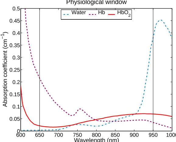
The technique relies on the “physiological window” (650-950 nm) (figure 1.1) where the photon propagation in the tissue is dominated by scattering rather than absorption [3]. In this part of the spectrum , as it is shown in figure 1.2, light experiences many scattering events and can penetrate several centimeters (>5 cm) into the tissue due to the low

(30)

probabilities of the detected photons from a particular source , has the so-called “banana shape” (figure 1.2).

6000 650 700 750 800 850 900 950 1000 0.05

0.1 0.15 0.2 0.25 0.3 0.35 0.4 0.45 0.5

Wavelength (nm)

Absorption coefficient (cm

−1

)

Physiological window

Water Hb HbO 2

Fig. 1.1 Absorption (µa) spectra of water, deoxy- and oxy-hemoglobin in

part of visible and near infrared range. The inset shows the “physiolog-ical window” where the absorption is relatively low and photon propa-gation is dominant by scattering events and photons can penetrate deep in the tissue.

Furthermore, in the “physiological window” there are clear features in the absorption spectra which enables us to estimate the chromophores concentrations (such as oxy- and deoxy-hemoglobin concentrations) and related them to total hemoglobin concentration (blood volume), blood oxygen saturation and oxygen consumption [4–7].

The main chromophores in this window are oxyhemoglobin (Hbo2),

deoxyhemoglobin (Hb), water (H2O) and lipids. For typical

[image:30.499.96.385.145.379.2]

(31)

3

(32)

microvasculature which makes the technology particularly unique as a noninvasive monitoring and imaging tool. Knowing the concentration of oxygenated and deoxygenated hemoglobin provided us with informa-tion about the blood oxygen saturainforma-tion which is an vital parameter and noninvasive measurement of it can provide valuable information over a wide range of medical conditions. For instance cerebral oxygenation monitoring has a great importance in minimizing secondary hypoxic and ischemic brain damage following severe head injury [8–11] or tumor hy-poxia is an crucial parameter in oncology [12–15] therefore knowledge about oxygen level has a high impact on cancer therapies [16, 17]. For instance figure 1.3 shows the difference in the reflected spectrum (mea-sured by the system described in the next chapters) of healthy tissue and tumor due to the hypoxia in the tumor. In hypoxic tissue (tumor) there is an absorption peak at ∼760 nm, which is the absorption peak

of deoxyhemoglobin.

600 650 700 750 800 850 900 950 1000

0.3 0.4 0.5 0.6

Wavelength (nm)

Tumor and healthy tissue spectrum

Normalized intensity

Hypoxic tumor spectrum Healthy tissue spectrum Fit for hypoxic tumor Fit for healthy tissue

Fig. 1.3 The difference in the reflected spectrum of healthy tissue and tumor due to the hypoxia in the tumor. In hypoxic tissue (tumor) there is an absorption peak at ∼760 nm, which is the absorption peak of

deoxyhemoglobin.

(33)

5

deoxy-hemoglobin concentration as well as water, lipid, bone miner-als and other desired tissue chromophores as the endogenous contrast species [18]. The sensitivity of measurement can be increased by the measurement of the concentration and lifetime of exogenous for exam-ple in the tumors [19–23]. Furthermore, from the speckle patterns of the multiply scattered light more information about dynamic proper-ties of tissue (blood flow) can be obtained by a relatively new NIR technique, called diffuse correlation spectroscopy (DCS) or diffuse wave spectroscopy (DWS) [24–31]. DCS has been validated against perfusion magnetic resonance imaging (MRI) [32–36], power Doppler ultrasound [37, 38], Doppler ultrasound [39–42], laser Doppler [43, 44], Fluorescent microspheres [45], and xenon-enhanced computed tomography [46].

Hybrid devices, combination of traditional NIRS devices and DCS, contain information from both static (total hemoglobin concentration and oxygen saturation) and dynamic (blood flow) properties of tissue which can provide us with information about metabolism of the tissue, which is an important clinical parameter.

Although diffuse optics is limited by its resolution, due to its ability to noninvasively measure vital physiological parameters, it has found a wide range of applications specially in neurology and oncology [47–55]. In neurology it has been applied mostly in brain functional spectroscopy and imaging [56–66], brain studies in animal models [35, 44, 45, 67– 77], stroke and brain damage investigation in adults and neonates [34, 40, 41, 78–87]. Wide range of neurological studies suggest that diffuse optics can play an important role not only as a complex research tool at the laboratory stage, but also as a powerful instrument for clinical applications.

(34)

demonstrated the feasibility of employing diffuse optics for detecting, imaging, characterizing and monitoring the hemodynamic changes in cancer.

Diffuse optics has been applied in experimental oncology to study tumors in animal samples for better understanding of cancer mecha-nisms and drug development [37, 38, 105–110]. Murine models are the most popular in vivo models in oncology study since they an

approx-imation of reality. Due to their similarity to the human in terms of genetics, anatomy and physiology, and ease of manipulation [111], they have been proven to be useful for novel cancer therapeutic strategies [112, 113].

My PhD is motivated mainly by application of diffuse optics for cancer studies to enhance the efficiency of new therapies and drugs. For this goal, I have applied hybrid diffuse optical devices to measure oxygen saturation, total hemoglobin concentration (blood volume), and blood flow which are important biomarkers of angiogenesis. Angiogen-esis, formation of new vessels, is a necessary process for tumor growth and metastasis. One of the new class of cancer drugs are angiogenesis inhibitors. These type of therapy does not follow the general rules of conventional chemotherapy. The successful translation of angiogenesis inhibitors to clinical application depends on better understanding of an-giogenesis in the tumor and the mechanisms of antiangiogenic therapies. As described, murine models are the good options for these investiga-tions. In order to study murine tumors, we have combined broadband near infrared spectroscopy (NIRS) and diffuse correlation spectroscopy (DCS) in a single hand-held self-calibrating probe for noninvasive, re-peated hemodynamic monitoring of murine tumors. The details of each device specification, probe design and validation tests are described in chapter 3.

(35)

fa-7

cility of IDIBELL (Bellvitge Biomedical Research Institute, Barcelona, Spain) for a multidisciplinary collaboration with Dr. Oriol Casanovas. We have monitored the hemodynamics of the murine tumors during antiangiogenic therapy for better understanding of tumors mechanisms again antiangiogenic therapies. The details of measurements and results are described in chapter 4.

To continue the cancer studies in clinical stage, we initiated a collab-oration with Dr. Alvaro Urbano at Hematology Department of Hospital Clínic de Barcelona in order to investigate the feasibility of applying diffuse optics in hematological malignancies. Most of the hematological malignancies originate in the bone marrow and alter its hemodynamics. Therefore, noninvasive methods that measure changes in hemodynamics induced by angiogenesis in the bone marrow have a potential impact on the earlier diagnosis, more accurate prognosis and in treatment moni-toring. To this end we have applied hybrid diffuse optical spectroscopy methods, time resolved spectroscopy (TRS) and DCS, to evaluate the feasibility of the noninvasive hemodynamics measurement in the healthy manubrium as a site of bone marrow. The measurement protocol and the details of the measured optical and physiology properties can be found in chapter 5.

(36)

pioneers of optical studies of bone. In this collaborative work we inves-tigate the cardiac cycle related pulsatile behavior of the absorption and scattering coefficients of diffuse light and the corresponding alterations in hemoglobin concentrations in the human patella. The physiological origin of the observed signals was confirmed by applying a thigh cuff. Moreover, we have investigated the optical and physiological proper-ties of the patella bone and their changes in response to arterial cuff occlusion. The details of this study is presented in chapter 6.

As it is described, I have performed optical measurements on hu-man and animal by hybrid (NIRS-DCS) devices. Can we utilize the full set of information available from multi-distance DCS measurements for better absolute quantification instead of hybrid devices? This question led me to develop a new algorithm using multi-distance DCS for simul-taneous measurement of absorption and scattering coefficient as well as blood flow index. The fitting is validated against numerical data, tissue simulating phantoms, and in-vivo measurements. The multi-distance

(37)

Chapter 2 Theoretical background

2.1 Light propagation in tissues

The propagation of the photons in tissues is mainly affected by scatter-ing rather than absorption. In this highly scatterscatter-ing medium few length scales are important: “scattering length” which corresponds to the typ-ical distance traveled by photons before they scatter and its reciprocal is named scattering coefficient (µs). The longer distance, “transport

mean-free path”, ltr, is the typical distance traveled by photons before

their direction is randomized. The reciprocal of the photon transport mean-free path is called the reduced scattering coefficient µs′ = 1/ltr.

The absorption length in tissue corresponds to the typical distance traveled by a photon before it is absorbed; its reciprocal, the absorp-tion coefficient, is denoted by µa. All three of these length scales are

wavelength-dependent [2].

Through this manuscript the light propagation in tissue is described

by “diffusion equation” where the photon fluence rate, Φ(ρ, t) (photons/[cm2_s]),

obeys the diffusion equation [123–125]:

∇ ·(D(ρ)∇Φ(ρ, t))−νµa(ρ)Φ(ρ, t)−

∂Φ(ρ, t)

(38)

This photon diffusion equation is valid when the radiance is nearly isotropic. This isotropy is achieved when µs′ ≫µa and and when

pho-ton propagation distances within the medium are large relative to ltr

that needs optode distance (ρ = |ρ|) to be more than 3ltr. In

addi-tion, the assumptions of isotropic source, slow temporal flux variations, and rotational symmetry should be valid [126]. Here, ν is the speed of

light in the medium (cm/s) and D = ₃₍_µ ν

a+µs′) is the photon diffusion

coefficient. To apply the photon diffusion equation the diffused light is detected at a known distance from the source.

2.2 Source types

One can categorize near infrared spectroscopy (NIRS) methods based on the source type. Three types of light sources are used in diffuse optics as it is shown in figure 2.1: continuous wave, intensity modulated and time pulsed.

The simplest source type is CW, where the intensity remains con-stant over time [37, 38, 43, 44, 50, 58, 68–70, 74, 80, 91, 92, 95, 97, 105– 109, 127–137]. CW measurements are simple and fast but they contain low amount of information. By single continuous wave (CW) measure-ment one can measure effective attenuation of medium but contribution of µa and µs′ cannot readily be decoupled.

Intensity modulated sources are more complex but also provide more information about the medium [35, 41, 45, 77, 85, 89, 116, 117, 119, 130, 132, 138–144]. In frequency domain (FD) measurements light in-tensity of the source is modulated with a frequency in order of 100 MHz or larger, up to ∼1 GHz, producing a diffusive wave in the medium

(39)

2.3 Diffuse photon density waves (DPDW) 11

Intens

ity _P0

P(r)

log(Intensity)

Intens

ity

Time Time(ns) Time(ns)

Input Input

output

Continous wave Frequency domain Time domain

Fig. 2.1 Three types of sources that are deployed to measure optical properties of medium. [Left] continuous wave (CW) is the simplest method that measures the intensity drop at a specific distance from the source. P0 is the intensity of the incident light and P(r) is detected

intensity at distance r from the source. [Middle] Frequency domain that delivers intensity modulated light to the medium and measures the phase shift (θ) and intensity drop of the detected light. [Right] Time

resolved spectroscopy (TRS) that shoots a narrow pulse to the medium and measures the broadening of the pulse.

source-detector separations provide simultaneous determination of µa

and µs′. Time-domain technique (time resolved spectroscopy, TRS) is

Fourier transform of frequency modulated measurement and it contains the same information content as FD measurement which is scanned over the wide range of modulation frequencies present in the pulse [51, 75, 90, 114, 145–157]. Due to multiple scattering in tissues the pulse temporally broadens. The information about optical properties of tissue can be extracted from the broadening of the detected light.

2.3 Diffuse photon density waves (DPDW)

The following theoretical discussion will be given in the frequency do-main (assumption of ω = 0 will be CW formulation), with the

(40)

in a turbid medium is intensity modulated, with “ac” and “dc” com-ponents (Sac and Sdc), the photon fluence will oscillate at the same

frequency. This small but measurable traveling wave disturbance of the light energy density is referred to as a diffuse photon density wave that oscillate at the same angular frequency as the source. [138, 158, 159]. The source term can be written as S(ρ, t) =Sdc(ρ) +Sac(ρ)e−iwt.

These ac solutions that oscillate at the same angular frequency as the source will have the following general form:

Φac(ρ, t) =U(ρ)e−iwt. (2.2)

By substituting equation 2.2 to diffusion equation (equation 2.1) we have:

∇ ·(D(ρ)∇U(ρ))−(νµa(ρ)−iω)U(ρ) = −νS(ρ, t)),

which for the homogeneous medium will be simplified to:

(∇2₋_k2₎_U₍_ρ_{) =} ₋ν

DSac(ρ).

The fluence rate of DPDW [2] in infinite geometry is:

U(ρ) = νSac

4πDρexp(−kρ). (2.3)

In equation 2.3, k is a complex wavevector k = kr + iki:

kr = ( νµa

2D)

1/2

[(1 + [ ω

νµa

]2₎1/2_{+ 1]}1/2_, _(2.4)

ki =−( νµa

2D)

1/2

[(1 + [ ω

νµa

]2₎1/2₋_1]1/2_. _(2.5)

(41)

of modulation frequency. The higher modulation frequency the larger wavevector. The dependency ofkrand ki on modulation frequency is

il-lustrated in figure 2.2. Writing the fluence rate in the formU(r) = Aeiθ_,

0 250 500 750 1000 1.6 1.8 2 2.2 2.4 2.6 K r (cm −1 ) Frequency (MHz) n = 1.33

ρ = 2.5 (cm)

µ_s′ = 10 (cm−1)

µ_a = 0.1 (cm−1)

0 250 500 750 1000 0 0.5 1 1.5 2 Frequency (MHz) K i (cm −1 )

Fig. 2.2 The dependency of real and imaginary parts of diffuse wave density wavevector (kr, ki) on modulation frequency (ω).

the determination of the change in wave amplitude, A, and wave phase,

θ, with distance from the source enables experimenters to extract µa

and µs′ of the turbid medium.

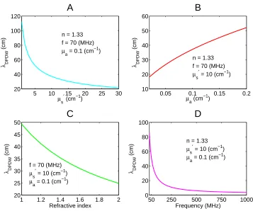
DPDWs have been demonstrated to exhibit several familiar wave-like properties including diffraction, refraction, interference and dispersion [159–162]. Figure 2.4 shows the dependency of DPDW’s wavelength on optical properties of the medium as well as its intensity modulation. While its wavelength, λDP DW, has direct relation with the absorption

coefficient (µa) of the medium, it has inverse relation with reduced

scat-tering coefficient (µs′), ratio of index of refraction to the outside (n) and

modulation frequency (ω).

(42)

source-0.5 1 1.5 2 2.5 3

−4 −3 −2 −1 0

Infinite

ln(

ρ

A(

ρ

))

ρ (cm)

Slope = −k

r Slope = −k

i

0.5 1 1.5 2 2.5 3 10 25

Phase(

°

)

ρ (cm)

Fig. 2.3 The phase shift,(green dashed line), and ln(Aρ), (blue solid

line), are plotted as the function of distance from the source in an in-finite turbid medium. The slopes reveal −ki and −kr (effective

attenu-ation coefficient, µef f), from which µa and µs′ can be calculated using

(43)

5 10 15 20 25 30 20 40 60 80 100 120 λ DPDW (cm)

µ_s′ (cm−1) n = 1.33 f = 70 (MHz)

µ_a = 0.1 (cm−1)

A

0.05 0.1 0.15 0.2 10 20 30 40 50 60 λ DPDW (cm)

µ_a (cm−1) n = 1.33 f = 70 (MHz)

µ s

′_{= 10 (cm}−1₎

B

1 1.2 1.4 1.6 1.8 2 20 25 30 35 40 45 50 λ DPDW (cm) Refractive index f = 70 (MHz)

µ_s′ = 10 (cm−1)

µ_a = 0.1 (cm−1)

C

50 250 500 750 1000 0 20 40 60 80 100 λ DPDW (cm) Frequency (MHz) n = 1.33

µ_s′ = 10 (cm−1)

µ_a = 0.1 (cm−1)

D

Fig. 2.4 The dependency of DPDW wavelength (λDP DW) on optical

properties of the medium and modulation frequency. [A] The reverse relation of DPDW’s wavelength and reduced scattering coefficient (µs′)

of the medium. [B] In the medium with higher absorption (µa), the

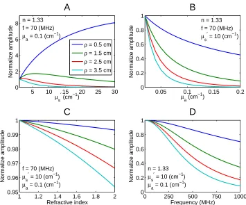
[image:43.499.74.431.145.443.2]

(44)

detector separations on the optical properties of tissue. In figure 2.5-A the relation between amplitude and µs′ is presented. In small values

of µs′ and small source-detector separations increase of µs′ lead to rise

in amplitude. While in largerµs′ and larger source-detector separations

higherµs′ results to lower amplitude. Figure 2.5-B shows the reverse

re-lation between absorption in the medium and the amplitude of DPDW. Similarly, Figure 2.5-c shows increase in ratio of index of refraction lead to decrease in intensity. Finally, the amplitude The amplitude decreases with increase of modulation frequency. (figure 2.5-D).

Due to multiple scattering in tissues by getting further from the source the phase increases. The dependency of phase on the medium optical properties as well as source modulation frequency over different source-detector separations is demonstrated in figure 2.6. While phase has reverse relation with the absorption coefficient (µa) of the medium,

it has direct relation with reduced scattering coefficient (µs′), index of

refraction (n) and modulation frequency (ω).

2.4 Green’s function solution to diffusion

equation for semi-infinite boundary

con-ditions

In NIRS, the most commonly used model approximate tissue as a ho-mogeneous semi-infinite medium. In order to find the diffusion equation Green’s function we have used method of images (figure 2.7). The ex-trapolated zero boundary condition is satisfied by introducing a negative image point source at zs = −(2zb +ltr). The fluence rate curve is

(45)

2.4 Green’s function solution 17

5 10 15 20 25 30 0 2 4 6 8 Normalize amplitude

µ_s′ (cm−1) n = 1.33

f = 70 (MHz)

µ_a = 0.1 (cm−1)

A

ρ = 0.5 cm

ρ = 1.5 cm

ρ = 2.5 cm

ρ = 3.5 cm

0.05 0.1 0.15 0.2 0 0.2 0.4 0.6 0.8 1 Normalize amplitude

µ_a (cm−1) n = 1.33 f = 70 (MHz)

µ_s′ = 10 (cm−1)

B

1 1.2 1.4 1.6 1.8 2 0.95 0.96 0.97 0.98 0.99 1 Normalize amplitude Refractive index f = 70 (MHz)

µ_s′ = 10 (cm−1)

µ_a = 0.1 (cm−1)

C

0 250 500 750 1000 0 0.2 0.4 0.6 0.8 1 Normalize amplitude Frequency (MHz) n = 1.33

µ_s′ = 10 (cm−1)

µ_a = 0.1 (cm−1)

D

Fig. 2.5 The dependency of amplitude of different source-detector sep-arations on the optical properties of tissue. [A] The relation between amplitude andµs′: in small values ofµs′ and small source-detector

sep-arations increase ofµs′ lead to rise in amplitude. While in largerµs′ and

larger source-detector separations higherµs′ results to lower amplitude.

[image:45.499.75.430.125.420.2]

(46)

5 10 15 20 25 30 0 10 20 30 40 50 60 Phase ( ° )

µ_s′ (cm−1) n = 1.33

f = 70 (MHz)

µ_a = 0.1 (cm−1)

A

0.05 0.1 0.15 0.2 0 20 40 60 80 Phase ( ° )

µ_a (cm−1)

B

n = 1.33 f = 70 (MHz)

µ_s′ = 10 (cm−1)

ρ = 0.5 cm

ρ = 1.5 cm

ρ = 2.5 cm

ρ = 3.5 cm

1 1.2 1.4 1.6 1.8 2 0 10 20 30 40 50 60 Phase ( ° ) Refractive index f = 70 (MHz)

µ_s′ = 10 (cm−1)

µ_a = 0.1 (cm−1)

C

0 250 500 750 1000 0 100 200 300 400 Phase ( ° ) Frequency (MHz) n = 1.33

µ_s′ = 10 (cm−1)

µ_a = 0.1 (cm−1)

D

Fig. 2.6 The dependency of phase on the medium optical properties and source modulation frequency over different source-detector separations. [A] Phase has direct relation with the reduced scattering coefficient (µs′)

[image:46.499.65.415.146.441.2]

(47)

solution to diffusion equation for semi-infinite boundary conditions[2].

G(ρ) = 1

4π[

exp(−kr1)

r1

− exp(−krb)

rb ] (2.6)

where:

r1 =

q ρ2₋_l

tr2 rb =

q ρ2+ (_l

tr+ 2zb)2 ltr =

1

µs′ zb = 2ltr

1 +Ref f

1−Ref f

k =

s

(µav−iw) D

D = ν

(µa+µs′)

Air

Tissue

-zb

-(2zb+ ltr) ltr

Image (–) Source (+)

Extrapolated Boundary

Fluence Rate Φ

z

Fig. 2.7 The extrapolated zero boundary condition is satisfied by intro-ducing a negative image point source at zs = −(2zb +ltr). The fluence

[image:47.499.92.422.114.545.2]

(48)

Here ρ is distance between source and detector, w is the intensity

modulation frequency. ltr is the mean distance that photon propagation

direction becomes randomize. zb is the extrapolated zero boundary and

D is the photon diffusion coefficient. Ref f is the effective reflection

coefficient to account for the index mismatch between tissue and air. The absolute value of photon fluence is corresponding to amplitude and angle part is the detected phase. Equation 2.6 can be fit exactly, but in the approximation of ρ ≫ (ltr + 2zb). In this case the solution

simplifies to:

U(ρ) =A(ρ)eiθ(ρ),

ln(ρ2A(ρ)) =−krρ+ lnA0, (2.7)

θ(ρ) = −kiρ+θ0. (2.8)

The equations 2.7 and 2.8 makes it possible to fit exactly for ki and kr

and calculate µa and µs′. Figure 2.8 shows that the slope of ln(A(ρ)ρ2)

versus ρ in semi-infinite boundary conditions is kr. Similarly, the slope

of phase versus ρ is kr. In CW measurements where we do not have

information about the phase by exact fitting for kr one can have

infor-mation about effective attenuation coefficient (µef f).

Patterson et al. [147] described the analytical solution of the diffusion equation (equation 2.1 for TRS. They have shown that the reflectance in a semi-infinite homogeneous medium for the time domain is described by:

R(t, ρ) = (4 π D ν)−32 µ_s′−1t− 5

2 exp[−µ_aν t]exp

"

−ρ

2₊_µ

s′−2

4D ν t #

. (2.9)

Photon penetration depth In experiments the detection of light can

(49)

0.5 1 1.5 2 2.5 3

−4 −3 −2 −1 0

Semi−infinite

ln(

ρ

2 A(

ρ

))

ρ (cm)

Slope = −k

r Slope = −k

i

0.5 1 1.5 2 2.5 3 10 25

Phase(

°

)

ρ (cm)

Fig. 2.8 The phase (green dashed line) and ln(A(ρ)ρ2) (blue solid line)

are plotted as the function of distance from the source in semi-infinite boundary condition. The slopes reveal −ki and −kr (effective

attenu-ation coefficient, µef f), from which µa and µs′ can be calculated using

(50)

through this manuscript, reflection geometry has been deployed. In the reflection geometry the probed medium has a “banana” shape which is demonstrated in figure 2.9. The simulated medium has µa = 0.1 cm−1, µs′ = 10 cm−1 and ρ = 2.5 cm. As a rule of thumb, the mean light

[mm]

S

D

−20 −15 −10 −5 0 5 10 15 20

14 11 8 5 2

Fig. 2.9 The “banana patterns” showing the sampled volumes in the reflection geometry. As a rule of thumb, the mean light penetration depth in the reflection geometry is in the order of half of source-detector separation (ρ/2). The simulated medium has µa = 0.1 cm−1, µs′ = 10

cm−1 and _ρ= 2_.5 cm.

[image:50.499.64.418.182.490.2]

(51)

source-detector separation (ρ/2). In other words, the larger the

source-detector separation, the deeper volume is probed [163]. In figure 2.10, the probability of detecting photons below certain depths is shown. The absorption coefficient (µa) of the simulated medium is 0.1 (cm−1), and

reduced scattering coefficient (µs′) is 10 (cm−1). It illustrates that larger

optode distances have higher probability of photon detection in deeper volumes. For instance, in optode distance of 0.5 cm, just less than 2% of detected photons traveled deeper than 1 cm, in optode distances of 5 cm this quantity is 40%.

2 4 6 8 10 20 40 60 80 0

0.2 0.4 0.6 0.8 1

Depth (mm)

Probability of detecting photons

µ_a = 0.1 cm−1, µ

s

′_{= 10 cm}−1

ρ = 0.5 cm

ρ = 1.5 cm

ρ = 2.5 cm

ρ = 5.0 cm

(52)

2.5 Multi-wavelength spectroscopy for

de-termination of tissue chromophore

con-centrations

The tissue absorption depends linearly on the concentrations of tissue chromophores. In particular, the wavelength-dependent absorption co-efficient is given by equation 2.10.

µa(λ) = nc X

i

ϵi(λ)ci (2.10)

The sum is over the different tissue chromophores. and nc is the

number of chromophores assumed. ϵi(λ) is the wavelength-dependent

extinction coefficient of theithchromophore obtained from the literature

[164], and ci is the concentration of the ith chromophore. By equation

2.10 one can calculate concentration of oxygenated hemoglobin and de-oxygenated hemoglobin (cHbO2 and cHb). The total hemoglobin concen-tration (THC) is the sum of oxygenated and deoxygenated hemoglobin, i.e:

T HC =cHbO2 +cHb. (2.11)

The blood oxygen saturation can be determined by:

SO2 =

cHbO2

T HC ×100. (2.12)

(53)

2.6 Diffuse correlation spectroscopy (DCS) 25

2.6 Diffuse correlation spectroscopy (DCS)

DCS measures the temporal speckle fluctuations of the scattered light, that is sensitive to the motions of scatterers such as red blood cells (RBCs) which in turn could be used to estimate microvascular blood flow [24, 25, 29, 166–168]. [2, 26–28]. The motional dynamics of the medium can be determined by measurement of intensity autocorrela-tion from which the electric field autocorrelaautocorrela-tion funcautocorrela-tion (G1) can be

derived. The fluctuations of the speckles are primarily due to move-ment of scatterers. Therefore, faster motion of the scatterers can be indicated by faster fluctuations (i.e., more rapid decay of the intensity temporal autocorrelation function). The Green’s function solution of the correlation diffusion equation for semi-infinite boundary conditions is [2]:

G1(ρ, τ) = 3

µs′

4π [

exp(−K(τ)r1)

r1

− exp(−K(τ)rb)

rb

] (2.13)

Where τ is delay time, r1 and rb are described in section 2.4 and K(τ)

is:

K(τ) = q

3µaµs′ + 6µs′2κ2αDbτ . (2.14) α represents the fraction of photon scattering events that occur from

moving particles in the medium, κ is the wave-number of light in the

medium: 2π/λ. DCS instrumentation measures the intensity temporal

autocorrelation function, while the correlation diffusion equation applies to the electric field temporal autocorrelation function. To compare the-ory with experiment, the normalized intensity autocorrelation function (g2) must be related to the normalized electric field temporal

autocorre-lation (g1). This connection is through Siegert relation (equation 2.15).

g1(τ) =

s

g2(τ)−1

(54)

β is a constant determined primarily by the collection optics of the

experiment. β is approximately equal to _N1 where N is the number of

detected speckles/ modes. In most of DCS studies non-polarized sources (vertical and horizontal modes) and single mode fibers are used to collect the diffused light and in this caseβ ∼0.5 [169]. In experimental dataβ

can be measured from the g2 whenτ is near to zero. Thus, g1 is derived

from the experimentally measured g2 , and K2 is determined by fitting

to the temporal decay of g1 (for a given source-detector separation).

This information in addition to optical property information (µa, µs′,

n) provide us with determination about mean square displacement of scatterers (<△r2₍_τ₎_>_{). The brackets represent time-averages (for}

ex-periments) or ensemble averages (for calculations). Thus by measuring the temporal fluctuations of scattered light, one obtains quantitative in-formation about the particle motions. For the case of Brownian motion,

<△r2₍_τ₎ _>_{= 6}_D

bτ and for random flow, <△r2(τ) >=< △V2 > τ2 .

Here, Db is the particle diffusion coefficient and <△V2 >is the second

moment of the particle speed distribution. In the study of blood flow in the microvasculature the random flow model seems the trivial choice for the dynamics of RBCs. In practice, it has been found [32–38, 46] that the Brownian model,<△r2₍_τ₎_>_{= 6}_D

bτ, fits the observed

correla-tion decay curves better over a wide range of tissue types. It has been demonstrated in several DCS measurements that the fitted parameter

αDb (from the Brownian model) correlates well with blood flow values

measured by other modalities [32–45]. Therefore we have defined αDb

as the blood flow index (BFI).

Figure 2.11 demonstrates the effect of different parameters on the shape of autocorrelation curves. This plot suggest that error in assump-tion of tissue µa orµs′ will introduce error in fitted BFI [170].

Noise model for DCS: In the following chapters we have simulated

(55)

2.6 Diffuse correlation spectroscopy (DCS) 27

10−6 10−5 10−4 10−3 10−2 10−1 0 0.2 0.4 0.6 0.8 1 g 1

0.3 x 10−8 0.4 x 10−8 0.6 x 10−8 0.8 x 10−8 1.0 x 1.0−8 cm2/sec

10−6 10−5 10−4 10−3 10−2 10−1 0 0.2 0.4 0.6 0.8 1 g 1 0.5 cm 0.7 cm 1.0 cm 1.2 cm 1.5 cm

10−6 10−5 10−4 10−3 10−2 10−1 0 0.2 0.4 0.6 0.8 1 g 1

Delay time (sec)

0.001 0.040 0.100 0.500 1.000 cm−1

10−6 10−5 10−4 10−3 10−2 10−1 0 0.2 0.4 0.6 0.8 1

Delay time (sec)

g 1

05 cm−1 07 cm−1 10 cm−1 12 cm−1 15 cm−1

lower BFI lower ρ

higher µ

a lower µ_s’

Fig. 2.11 Effect of different parameters on the shape of field autocorrela-tion curve. Decrease in blood flow index (BFI), source-detector separa-tion (ρ) and scattering coefficient (µs′) as well as increase in absorption

coefficient (µa) will cause higher correlation therefore later drop of AC

[image:55.499.74.437.203.420.2]

(56)

theoretical intensity autocorrelation. The noise model for DCS measure-ments is developed by Zhou et al. [76]. It has adapted the noise model for fluorescence correlation spectroscopy developed by Koppel [171]. In a DCS experiment, the normalized field autocorrelation function decays exponentially ( g1(τ) = e−Γ τ ). The optical/mechanical properties of

medium and experimental conditions define the value of Γ. The

stan-dard deviation (σ(τ), noise) of the measured intensity AC,g2(τ), at each

delay time (τ) is estimated to be:

σ(τ) = qT /t "

β2(1 +e

−2Γ T_{)(1 +}_e−2Γ τ_{) + 2}_m₍₁₋_e−2Γ T₎_e−2Γ τ

1−e−2Γ T

#1

2

+ h

2< n >−1 β(1 +e−2Γ τ)+ < n >−2 (1 +βe−Γ τ)i

1 2

. (2.16)

In equation 2.16, T is the correlator bin time interval, m is the bin index corresponding to the delay timeτ . In our correlator the bin time

interval is T = 200 ns for the first 16 channels and is doubled every 8 channels afterwards. The average number of photons < n >within bin

time T (i.e. < n >= IT, where I is the detected photon count rate), t

(57)

Chapter 3 Hybrid broadband

NIRS-DCS instrumentation

for experimental oncology

3.1 Introduction

Murine models are the most popular in vivo models in oncology study

and by definition, are an approximation of reality. The major reason that mice are used is the similarity of mouse and human genetic and this greatly increased the value of animal models for research on human disorders specially cancer [111].

Genetically engineered mouse models have significantly contributed to the understanding of cancer biology. They have proven to be useful in clinical models in which novel therapeutic strategies are tested [112, 113].

(58)

vessels that penetrates into cancerous regions, supplying nutrients and oxygen and removing waste products [172–174]. The high metabolism and vascular supply make a contrast between cancerous and normal tissue hemodynamics.

By taking advantage of near infrared spectroscopy (NIRS) ability to map oxygen saturation and blood volume as well as diffuse correlation spectroscopy (DCS) for blood flow measurements, (look at section 2.5), we can study microvascular physiology noninvasively as opposed to the most common imaging modalities that allow probing of tumor morphol-ogy [6]. For example, metastatic cancers (when a cancer spreads from its original site to another area of the body, it is termed metastatic can-cer), in general, have higher metabolism and higher blood volume and by NIRS and DCS techniques we can find tissues with higher metabolism and distinguish metastatic tumors from benign ones.

Furthermore, monitoring the hemodynamics changes induced by ther-apies can provide valuable information about the outcome of therapy. This information can be used to personalize the therapeutic plan for each patient. Many techniques have aimed to monitor the cancer ther-apies [175–178]. This aspect of my research focuses on monitoring of cancer therapies where we postulate that physiological changes could be observed prior to morphological changes.

3.1.1 Cancer therapies and optimizing their

effi-ciency

(59)

3.1 Introduction 31

adjacent tissue or to spread to distant sites by microscopic metastasis often limits its effectiveness; chemotherapy, radiotherapy, phtodynamic therapy are prominent treatments.

Chemotherapy: It uses drugs to stop or slow the growth of cancer

cells to shrink the tumors. It is often applied before surgery (neoadju-vant) or after radiation therapy or surgery to destroy remaining cancer cells from radiation therapy or surgery [179–181]. Chemotherapy may have serious side effects such as: anemia (low red blood cell count) [182] which causes lack of oxygen circulating in the body, thrombocytope-nia (low platelet count) that may reason bruising or excessive bleeding, neutrogena (low white blood cell count) hair losses, eating and skin problems, etc. While certain cytotoxic side effects can be even life-threatening [183], under-dosing of patients, which may compromise the probability of cure for cancers that are curable with chemotherapy, is not acceptable. Because of the enormous consequences to cancer patients, maximizing the efficacy of chemotherapy is of prime importance.

Radiation therapy: It uses high energy radiation: X–ray, gamma,

neutrons, protons, etc. to kill cancer cells and shrink tumors [184, 185]. It has two kinds:

1. internal: it has internal source of radiation like radioactive mate-rial.

2. external: it has external source of radiation like X-ray.

(60)

Photodynamic therapy (PDT): Although this method is still mainly experimental, it is of particular interest for a photonics research group since it uses light activated drugs to destroy cells [187, 188]. In this method photosensitizer is injected to the patient. The interaction be-tween laser light and photosensitizer makes excited singlet oxygen which can destroy cells. There are important key components that need to be optimized, for example, the drug dose and the activating light dose. It is generally a difficult problem to predict how much light would be delivered into deep tissues.

Cancer therapy monitoring and enhancement Here I outline one

of our key goals which is to monitor cancer therapy to understand its fundamental effects on different types of tumors and physiological condi-tions as well as to suggest potential strategies that could then be tested on humans to optimize the treatment. Let’s take PDT as an exam-ple. The micro-vasculature is the primary mechanism to delivers the treatment drug to the remote parts of the tissues of interest, but the selectivity (in general, unless some targeting mechanism is used) is low and the drug can kill cancer cells as well as the normal tissue and blood vessels. In fact, the destruction of blood vessels to the cancerous regions is often the goal but it has a side-effect that it may stop the delivery of the drug to the cancer tissue prematurely, hence hindering the treat-ment. Monitoring the blood flow during the therapy can assist us to control this situation and we can “tune” the therapy so that the blood flow is maintained long enough to ensure adequate delivery of drug to the tumor. Monitoring of microvascular blood flow is possible by means of diffuse correlation spectroscopy. In radiation therapy and PDT, oxy-gen plays an important role in the therapy effect. Without oxyoxy-gen, the therapy is not effective and hence local, microvascular, monitoring of the oxygen is important. We can continuously measure the HbO2

(61)

3.2 Combination of NIRS and DCS in a single probe 33

oxygen locally. In the work by Yu et al. [37], it has been shown that by finding the optimum blood flow patterns during therapy and providing a feed-back mechanism to alter the light fluence/duration, we may be able to improve the efficiency of therapy. Since then similar effects have been observed in other tumor models and even was suggested in human trials of PDT [106, 109, 110, 131, 132, 142, 189].

3.2 Combination of broadband NIRS and

DCS in a single probe

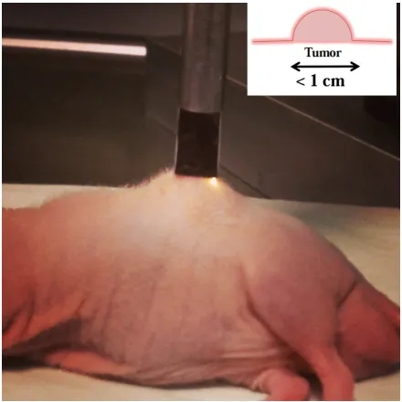
The murine tumors are small in size (< 1 cm in diameter) (figure 3.1) therefore to perform measurement on them the maximum distance be-tween source and detector can not be more than few millimeters (5 mm). Although time resolved spectroscopy (TRS) and frequency domain (FD) contain higher amount of information (look at figure 2.1), in such small source-detector separation the broadening of pulse in TRS and phase shift in FD is small and is difficult to be detected by current instru-mentation. Therefore, we have chosen multi-distance continuous wave (CW).

In single wavelength CW measurement one can not decouple µa and µs′, and we can just measure effective attenuation coefficient (which is

called k, kr or µef f). In order to decouple µa and µs′ we have used

broadband light source [37, 43, 58, 69, 70, 91, 92, 95, 97, 105–109, 127– 129, 131, 133–135, 137]. By broadband NIRS we can measure optical properties of tissue (µa, µs′) as well as concentration of oxygenated

hemoglobin (cHbO2), deoxygenated hemoglobin (cHb), total hemoglobin concentration (THC) and oxygen saturation (SO2) (for more details

(62)

[image:62.499.129.349.208.428.2]

(63)

3.3 Broadband near infrared spectroscopy 35

an important parameter for in-vivo studies.

3.3 Broadband near infrared spectroscopy

In the last decades several groups have applied broadband NIRS for experimental oncology in small animals.Weersink et al. [108] are one of the first groups who have used self-calibrating probe for broadband NIRS study. To increase the speed of measurements some groups have taken advantage of two-dimensional CCD cameras for gathering simul-taneous spectral and spatial information [105, 131]. The goal here was to develop an instrument with high information content (i.e. high quan-tification) while being easy to operate by a small probe that resembles a “pen” (figure 3.7). It should be operated by biomedical researchers. It takes advantage of white light and multi-track spectrometers for NIRS to acquire a relatively complete spectrum from multiple separations [37, 43, 58, 70, 92, 95, 97, 105–109, 127–129, 131, 133]. The goal is to acquire multi-spectral, multi-distance measurements to be used in an algorithm that uses both these aspects for both NIRS and DCS to re-cover the optical properties and blood flow accurately. Figure 3.2 shows that the light source is a broadband lamp. The light is delivered to the tissue through multi-mode fibers and the diffuse light is collected in dif-ferent distances from the source to a 2D spectrometer. The information about intensity on each wavelength/distance is transformed a computer for post-processing.

Light Source: We want to work in physiological window (650-1000

(64)

Fig. 3.2 The schematic of white-light device.The light source is a broad-band lamp. The light is delivered to the tissue through multi-mode fibers and the diffuse light is collected in different distances from the source to a 2D spectrometer. The information about intensity on each wavelength/distance is transformed to a computer for post-processing.

USA). It has an internal shutter which enables us to block white-light when we want to work with the DCS laser.

Spectrometer and CCD: We planned to image eight fibers on to

(65)

3.4 Diffuse correlation spectroscopy 37

95% at 700nm. (PIXIS: 400B-eXcelon , Princeton Instrument1_{). This}

CCD is a 1340 × 400 imaging array, with 20 × 20 microns pixels. We

can improve the resolution of spectrometer by increasing the intensity of grooves of grating. But grating with higher groove intensity can cover narrower spectral range, so there is a compromise between range of cov-ered spectra and resolution. Resolution also depends on size of entrance slit. Smaller slits makes higher resolution but the light which can enter is lower (lower level of signal). With bigger grating we can have better spatial and spectral separation. However, the cross-talk between fibers on CCD was also an important parameter for us. We need to have the cross talk less than 1% for 8 fibers with 200µm cores. Considering all

these parameters our final choice was Acton InSight-EPF from Princeton instruments with 150 g/mm grating which gives us a resolution about 5 nm covering 545-1055 nm.

3.4 Diffuse correlation spectroscopy

In this setup, DCS is employed for the measurement of blood flow. It has a single longitudinal mode laser as source(DL785-120-SO, 120mW, 785nm from Crystalaser); the coherence length (>15 m) of the laser is much longer than a typical photon path length. The laser light is delivered to the tissue through a multimode fiber with a core diameter of 200 µm (NA = 0.22). Due to necessity to detect single speckle, DCS

uses single mode fibers of 5.8 µm core diameters for collection. Photon

counting avalanche photodiodes (APDs) are used as detectors (SPCM-AQRH-14-FC, Pacer Internal) whose output is fed to a digital correlator (Correlator.com, NJ, USA) to obtain the autocorrelation functions. The schematic of DCS device is shown in figure 3.3.

1Data is retrieved from Princeton Instrument website. Last access on

30/July/2014:

Hybrid diffuse optics for monitoring of tissue hemodynamics with applications in oncology

PARISA FARZAM

Advisor:

Turgut Durduran

Hybrid diffuse optics for monitoring

of tissue hemodynamics with

applications in oncology

D O C T O R A L T H E S I S I N P H O T O N I C S

I C F O B A R C E L O N A 2 0 1 4

Doctor of Philosophy in Photonics

Institute of Photonic Sciences (ICFO)

Hybrid diffuse optics for

monitoring of tissue hemodynamics

with applications in oncology

by

Parisa Farzam

Ph.D. Dissertation

Declaration

Acknowledgements

Abstract

Hybrid diffuse optics for

monitoring of tissue hemodynamics

with applications in oncology

Parisa Farzam

Resumen

Óptica difusa híbrida para la

monitorización de la hemodinámica de los

tejidos con aplicaciones en oncología

Parisa Farzam

Table of contents

List of figures

List of tables

Nomenclature

Chapter 1

Introduction

Tumor and healthy tissue spectrum

Chapter 2

Theoretical background

2.1

Light propagation in tissues

2.2

Source types

2.3

Diffuse photon density waves (DPDW)

A

B

C

D

2.4

Green’s function solution to diffusion

equation for semi-infinite boundary

con-ditions

A

B

C

D

A

B

C

D

Air

Tissue

Fluence Rate Φ

z

S

D

2.5

Multi-wavelength spectroscopy for

de-termination of tissue chromophore

con-centrations

2.6

Diffuse correlation spectroscopy (DCS)

Chapter 3

Hybrid broadband

NIRS-DCS instrumentation

for experimental oncology

3.1

Introduction

3.1.1

Cancer therapies and optimizing their

_{Parisa Farzam}