Essays on Empirical Asset Pricing

Texto completo

(1)Universitat Autónoma de Barcelona. Doctoral Thesis. Essays on Empirical Asset Pricing. Author: Xiang Zhang. Supervisor: Abhay Abhyankar. A thesis submitted in fulfillment of the requirements for the degree of Doctor of Philosophy in the subject of Economics in the The International Doctorate in Economic Analysis Program Departament d’Economia i d’História Económica. June 2013.

(2) UNIVERSITAT AUTÓNOMA DE BARCELONA. Abstract Thesis Advisor: Professor Abhay Abhyankar Departament d’Economia i d’História Económica Doctor of Philosophy Essays on Empirical Asset Pricing by Xiang Zhang.

(3) ii This thesis consists of three essays on empirical asset pricing around three themes: evaluating linear factor asset pricing models by comparing their misspecified measures, understanding the long-run risk on consumption-leisure to investigate their pricing performances on cross-sectional returns, and evaluating conditional asset pricing models by using the methodology of dynamic cross-sectional regressions. The first chapter is “Comparing Asset Pricing Models: What does the Hansen–Jagannathan Distance Tell Us?”. It compares the relative performance of some important linear asset pricing models based on the Hansen–Jagannathan (HJ) distance using data over a long sample period from 1952–2011 based on U.S. market. The main results are as follows: first, among return-based linear models, the Fama–French (1993) [1] five-factor model performs best in terms of the normalized pricing errors, compared with the other candidates. On the other hand, the macro-factor model of Chen, Roll, and Ross (1986) [2] five-factor is not able to explain industry portfolios: its performance is even worse than that of the classical CAPM. Second, the Yogo (2006) [3] non-durable and durable consumption model is the least misspecified, among consumption-based asset pricing models, in capturing the spread in industry and size portfolios. Third, the Lettau and Ludvigson (2002) [4] scaled consumption-based CAPM (C-CAPM) model obtains the smallest normalized pricing errors pricing gross and excess returns on size portfolios, respectively, while Santos and Veronesi (2006) [5] scaled C-CAPM model does better in explain the return spread on portfolios of U.S. government bonds. The second chapter (“Leisure, Consumption and Long Run Risk: An Empirical Evaluation”) uses a long-run risk model with non-separable leisure and consumption, and studies its ability to price equity returns on a variety of portfolios of U.S. stocks using data from 1948–2011. It builds on early work by Eichenbaum et al. (1988) [6] that explores the empirical properties of intertemporal asset pricing models where the representative agent has utility over consumption and leisure. Here we use the framework in Uhlig (2007) [7], that allows for a stochastic discount factor with news about longrun growth in consumption and leisure. To evaluate our long-run model, we assess its performance relative to standard asset pricing models in explaining the cross-section of returns across size, industry and value-growth portfolios. We find that the long-run consumption-leisure model cannot be rejected by the J–statistic and it does better than the standard consumption-based CAPM, the Yogo durable consumption and Fama– French three-factor models. We also rank the normalized pricing errors using the HJ distance: our model has a smaller HJ distance than other candidate models. Our paper is the first, as far as we are aware, to use leisure data with adjusted working hours as a measure of leisure i.e., defined as the difference between a fixed time endowment and the observable hours spent on working, home production, schooling, communication, and personal care (Yang (2010) [8])..

(4) iii The third essay: “Empirical Evaluation of Conditional Asset Pricing Models: An Economic Perspective” uses dynamic Fama–MacBeth cross-sectional regressions and tests the performance of several important conditional asset pricing models when allowing for time-varying price of risk. It compares the performance of conditional asset pricing models, in terms of their ability to explain the cross-section of returns across momentum, industry, value-growth and government bond portfolios. We use the new methodology introduced by Adrian et al. (2012) [9]. Our main results are as follows: first we find that the Lettau and Ludvigson (2001) conditional model does better than other models in explaining the cross-section of momentum and value–growth portfolios. Second we find that the Piazessi et al. (2007) consumption model does better than others in pricing the cross-section of industry portfolios. Finally, we find that in the case of the cross-section of risk premia on U.S. government bond portfolios the conditional model in Santos and Veronesi (2006) outperforms other candidate models. Overall, however, the Lettau and Ludvigson (2001) model does better than other candidate models. Our main contributions here is using a recently developed method of dynamic Fama–MacBeth regressions to evaluate the performance of leading conditional CAPM (C-CAPM) models in a common set of test assets over the time period from 1951–2012..

(5) Acknowledgements I became interested in empirical asset pricing as a master student at UAB while taking the course taught by Abhay Abhyankar. Working on a senior thesis on that topic, I had read many related papers and became captivated by the intimate connection between theory and evidence at the frontier of empirical asset pricing. Abhay has led me step by step in the process of becoming an academic: first equipping me with the necessary tools through a research assistantship, then teaching me to carry out a research project from start to finish through a joint paper (Chapter 1), and finally navigating me through my “job market paper” (Chapter 2) and the third essay (Chapter 3). I thank Abhay for his father-like kindness and strict requirements for my research. Michael Creel has contributed to my intellectual development, particularly in econometrics. What began as a tutor of mine in my first year developed into a three-year research on application of the general moment estimator. His helps led me to write Chapter 1 and Chapter 2 of the thesis. I thank Michael for his constant encouragement and support during my graduate studies. Jordi Caballé and Francisco Peñaranda have given me invaluable guidance and support on the work contained in the thesis. I also want to thank others who have provided helpful feedback on parts of the thesis. Chapter 1 has benefited from comments by Cesare Robotti, Raymond Kan, Motohiro Yogo, and Rosario Crinó, and seminar participants at Arne Ryde Workshop, RIEM, IFS in Southwestern University of Finance and Economics, QQE 2011, EEFS 2011, and Rimini Quantitative Finance Workshop. Chapter 2 has benefited from comments by Phil Dybvig, Mark Loewenstein, Michael Brennan, Albert Marcet, Hossein Asgharian, Marvin Goodfriend, Tan Wang, Harald Uhlig and seminar participants at Centre for Finance in University of Gothenburg, International 2012 Paris Finance Meeting, SAEe2012, Institute of Financial Studies, RIEM in Southwestern University of Finance and Economics and Arne Ryde Workshop. Chapter 3 has benefited from comments by Abhay Abhyankar and Michael Creel. I am very grateful for financial support through the Spanish Ministry of Science and Innovation through grant ECO2008-04756 (Grupo Consolidado-C) and FEDER in 20092013. Without the generous support, I would not have been able to complete my doctoral work in three years. What I will most miss about graduate school are the daily interactions with interesting and nice colleagues. In particular, I will miss the not always productive conversations with Pinghan Liang, Dimitrios Bermperoglou, and Emanuel Alfranseder. I learned a lot about economics and life from these guys. Special thanks to Jingwen Liu for bearing the iv.

(6) v downs with me through the final two years. Lastly, I thank my parents for a constant source of wisdom and encouragement..

(7) To my parents, Kai Zhang and Yixiu Lv, and my daughter, Elisa Xinyuan Zhang. vi.

(8) Contents Abstract. i. Acknowledgements. iv. List of Tables. ix. List of Figures. x. 1 Comparing Asset Pricing Models: What does the Hansen–Jagannathan Distance Tell Us? 1.1 Introduction and Motivation . . . . . . . . . . . . . . . . . . . . . . . . . . 1.2 Test Methodology . . . . . . . . . . . . . . . . . . . . . . . . . . . . . . . 1.2.1 Hansen–Jagannathan Distance . . . . . . . . . . . . . . . . . . . . 1.2.2 Modified Hansen–Jagannathan Distance . . . . . . . . . . . . . . . 1.2.3 Constrained Hansen–Jagannathan Distance . . . . . . . . . . . . . 1.2.4 Testing for Multiple Comparisons . . . . . . . . . . . . . . . . . . . 1.3 Description of the Candidate Models . . . . . . . . . . . . . . . . . . . . . 1.3.1 Return-Based Linear Factor Asset Pricing Models . . . . . . . . . 1.3.2 Consumption-Based Linear Factor Asset Pricing Models . . . . . . 1.3.3 Linear Scaled Factor Asset Pricing Models . . . . . . . . . . . . . . 1.4 Preliminary Analysis of Data . . . . . . . . . . . . . . . . . . . . . . . . . 1.4.1 Data Descriptions . . . . . . . . . . . . . . . . . . . . . . . . . . . 1.4.2 Empirical Results on Return-Based Models . . . . . . . . . . . . . 1.4.3 Empirical Results on Consumption-Based Models . . . . . . . . . . 1.4.4 Empirical Results on Scaled Consumption-Based Models . . . . . . 1.4.5 Economic Interpretations . . . . . . . . . . . . . . . . . . . . . . . 1.5 Conclusions . . . . . . . . . . . . . . . . . . . . . . . . . . . . . . . . . . .. 1 1 3 3 4 4 5 6 6 7 8 9 9 9 10 11 12 13. 2 Leisure, Consumption and Long Run Risk: An Empirical Evaluation 2.1 Introduction . . . . . . . . . . . . . . . . . . . . . . . . . . . . . . . . . . . 2.2 Stylized Facts . . . . . . . . . . . . . . . . . . . . . . . . . . . . . . . . . . 2.2.1 Leisure and Consumption . . . . . . . . . . . . . . . . . . . . . . . 2.2.2 Leisure, Consumption and Asset Returns . . . . . . . . . . . . . .. 25 25 26 26 28. vii.

(9) Contents 2.3. 2.4. 2.5. 2.6. viii. The Model . . . . . . . . . . . . . . . . . . . . . . . . . . . . 2.3.1 Epstein–Zin Preferences with Leisure . . . . . . . . . . 2.3.2 Log-linearizing the First Order Conditions . . . . . . . 2.3.3 The Stochastic Discount Factor (SDF) . . . . . . . . . 2.3.4 The Return–Risk in the Model . . . . . . . . . . . . . Test Methodology . . . . . . . . . . . . . . . . . . . . . . . . 2.4.1 State of the Economy . . . . . . . . . . . . . . . . . . 2.4.2 News Shock Identification . . . . . . . . . . . . . . . . 2.4.3 Data Description . . . . . . . . . . . . . . . . . . . . . 2.4.3.1 Asset Returns . . . . . . . . . . . . . . . . . 2.4.3.2 Consumption . . . . . . . . . . . . . . . . . . 2.4.3.3 Leisure . . . . . . . . . . . . . . . . . . . . . Basic Results . . . . . . . . . . . . . . . . . . . . . . . . . . . 2.5.1 Data Analysis . . . . . . . . . . . . . . . . . . . . . . . 2.5.1.1 A Linear-factor Asset Pricing Model . . . . . 2.5.1.2 Hansen–Jagannathan Distance and Multiple son Test . . . . . . . . . . . . . . . . . . . . . 2.5.2 Additional Robustness Checks . . . . . . . . . . . . . Concluding Remarks . . . . . . . . . . . . . . . . . . . . . . .. . . . . . . . . . . . . . . . . . . . . . . . . . . . . . . . . . . . . . . . . . . . . . . . . . . . . . . . . . . . . . . . . . . . . . . . . . . . . . . . . . . . . . . . . . . Compari. . . . . . . . . . . . . . . . . .. . . . . . . . . . . . . . . .. 29 29 31 32 34 35 35 36 39 39 39 40 40 40 41. . 44 . 44 . 45. 3 Empirical Evaluation of Conditional Asset Pricing Models: nomic Perspective 3.1 Introduction . . . . . . . . . . . . . . . . . . . . . . . . . . . . . 3.2 The Model . . . . . . . . . . . . . . . . . . . . . . . . . . . . . 3.3 Test Methodology . . . . . . . . . . . . . . . . . . . . . . . . . 3.4 Data and Conditional Variables . . . . . . . . . . . . . . . . . . 3.5 Basic Empirical Results . . . . . . . . . . . . . . . . . . . . . . 3.5.1 The Main Result . . . . . . . . . . . . . . . . . . . . . . 3.5.2 Robustness Check . . . . . . . . . . . . . . . . . . . . . 3.5.2.1 Other Conditional Variables . . . . . . . . . . 3.5.2.2 Conditional Variables and the Business Cycle . 3.6 Conclusion . . . . . . . . . . . . . . . . . . . . . . . . . . . . .. . . . . . . . . . .. . . . . . . . . . .. . . . . . . . . . .. . . . . . . . . . .. . . . . . . . . . .. . . . . . . . . . .. 67 67 69 71 74 75 75 78 78 79 80. A Appendix on Chapter 1 A.1 Sample Estimates on Hansen–Jagannathan (HJ) Distance . A.2 Testing Hansen–Jagannathan Distance . . . . . . . . . . . . A.2.1 Testing Constrained Hansen–Jagannathan Distance A.3 Entropy and the Filtered Pricing Kernel . . . . . . . . . . . A.3.1 The Least Misspecified SDF and Economic Cycles . A.4 A Nonparametric Method for Canonical Valuation . . . . .. . . . . . .. . . . . . .. . . . . . .. . . . . . .. . . . . . .. . . . . . .. 90 90 91 92 93 95 97. . . . . . .. . . . . . .. An Eco-. B Appendix on Chapter 2 102 B.1 Unemployment . . . . . . . . . . . . . . . . . . . . . . . . . . . . . . . . . 102 B.2 Home production . . . . . . . . . . . . . . . . . . . . . . . . . . . . . . . . 103 Bibliography. 107.

(10) List of Tables 1.1 1.2 1.3 1.4 1.5 1.6 1.7 1.8 1.9. Return-based Models via HJ and Modified HJ Distance . . . . Return-based Models via Unconstrained HJ Distance . . . . . . Return-based Models via Constrained HJ Distance . . . . . . . Consumption-based Models via HJ and Mod. HJ Distance . . Consumption-based Models via Unconstrained HJ Distance . . Consumption-based Models via Constrained HJ Distance . . . Cond. Consumption-based Models via HJ and Mod. HJ Dist. Cond. Consumption-based Models via Unconst. HJ Dist. . . . Cond. Consumption-based models via Constrained HJ Dist. . .. . . . . . . . . .. 15 16 17 18 19 20 21 22 23. 2.1 2.2 2.3 2.4 2.5 2.6 2.7. 47 48 49 50 51 52. 2.11 2.12 2.13 2.14. An Initial Leisure Analysis . . . . . . . . . . . . . . . . . . . . . . . . An Initial Consumption Analysis . . . . . . . . . . . . . . . . . . . . Exposure to Benchmark Candidates (Multivariate) . . . . . . . . . Exposure to Benchmark Candidates (Univariate) . . . . . . . . . . Exposure to Long-run Three Factors (Multivariate) . . . . . . . . Exposure to Long-run Three Factors (Univariate) . . . . . . . . . Cross-section Results Without Constant on Fama–French 25 Portfolios (Multivariate) . . . . . . . . . . . . . . . . . . . . . . . . . . Cross-section Results Without Constant on Fama–French 25 Portfolios (Univariate) . . . . . . . . . . . . . . . . . . . . . . . . . . . Cross-section Results With Constant on Fama-French 25 Portfolios (Multivariate) . . . . . . . . . . . . . . . . . . . . . . . . . . . . . Cross-section Results With Constant on Fama–French 25 Portfolios (Univariate) . . . . . . . . . . . . . . . . . . . . . . . . . . . . . . GMM Results on Fama–French 25 Portfolios . . . . . . . . . . . . . Hansen–Jagannathan Distance Comparisons . . . . . . . . . . . . . R2 , Alpla, and χ2 Tests on Fama–French 25 Size and Momentum R2 , Alpla, and χ2 Tests on 30 Industry-sorted . . . . . . . . . . . .. 3.1 3.2 3.3 3.4 3.5 3.6 3.7 3.8. Lettau–Ludvigson - Price of Risk Estimates . . . . . . . . . Lustig–Van Nieuwerburgh - Price of Risk Estimates . . . . Piazzesi–Schneider–Tuzel - Price of Risk Estimates . . . . . Santos–Veronesi - Price of Risk Estimates . . . . . . . . . . The Default Rate in CAPM - Price of Risk Estimates . . . The Default Rate in CCAPM- Price of Risk Estimates . . The Dividend Yields in CAPM - Price of Risk Estimates . The Dividend Yields in CCAPM - Price of Risk Estimates. 2.8 2.9 2.10. ix. . . . . . . . .. . . . . . . . .. . . . . . . . .. . . . . . . . .. 53 54 55 56 57 58 59 60 81 82 83 84 85 86 87 88.

(11) List of Figures 1.1. Hansen–Jagannathan Distance . . . . . . . . . . . . . . . . . . . . . . 24. 2.1 2.2 2.3 2.4 2.5 2.6 2.7 2.8 2.9 2.10 2.11. Enjoyment of Various Activities in 1985 . . . . . . . . . . . Average Weekly Hours of Leisure . . . . . . . . . . . . . . . Non-durable Consumption and Services . . . . . . . . . . . The Growth on Hours of Leisure . . . . . . . . . . . . . . . The Growth on Non-durable Consumption and Services Leisure Growth and Equity Returns . . . . . . . . . . . . . Per Capita Consumption Growth and Equity Returns . . Correlation Analysis for Consumption . . . . . . . . . . . . Correlation Analysis for Leisure . . . . . . . . . . . . . . . . Impulse Responses Functions (Growth) . . . . . . . . . . . Impulse Responses Functions (Log Level) . . . . . . . . . .. 3.1. Conditional Variables . . . . . . . . . . . . . . . . . . . . . . . . . . . . 89. A.1 A.2 A.3 A.4 A.5. Fama–French Five-factor in Fama–French 25 Portfolios Fama–French Five-factor in FF 25 plus Gov. Bonds . . Yogo in 10 Deciles Portfolios . . . . . . . . . . . . . . . . . Lettau and Ludvigson in 30 Industry Portfolios . . . . . Santos and Veronesi in 30 Industry Portfolios . . . . . .. . . . . .. . . . . . . . . . . .. . . . . .. . . . . . . . . . . .. . . . . .. . . . . . . . . . . .. . . . . .. . . . . . . . . . . .. . . . . .. . . . . . . . . . . .. . . . . .. 61 61 62 62 62 63 63 64 65 65 66. 99 99 100 100 101. B.1 The Correlation between Leisure and the Unemployment . . . . . 105 B.2 Home Production, Leisure and Equity Returns . . . . . . . . . . . 105 B.3 Working, Home Production and Leisure . . . . . . . . . . . . . . . . 106. x.

(12) Chapter 1. Comparing Asset Pricing Models: What does the Hansen–Jagannathan Distance Tell Us? 1.1. Introduction and Motivation. The purpose of this paper is to compare the relative performance of some important linear asset pricing models based on the Hansen–Jagannathan (HJ) distance using data over a long sample period from 1952–2011 based on U.S. market. Such comparisons, in the prior literature (for example, Lettau and Ludvigson (2001)[10], Lustig and Van Nieuwerburgh (2005)[11], and Parker and Julliard (2005)[12]) rely on tests of pricing errors for individual models using purely statistical criteria such as Fama– MacBeth cross-sectional regression or the Hansen–Singleton J–statistics (1982). We see that most asset pricing models are rejected by these statistical tests: this is not surprising given that most of them are misspecified. Thus, such comparisons of individual models, even using the same test assets and data, does not help us to understand why the models fail. In contrast, the HJ measure is a test of the degree of misspecification from the “true” model that correctly prices the data. In this paper, we use this measure, based on new econometric methods proposed by Hansen and Jagannathan (1997) [13], which allow us to compare across models and to choose the one that prices the chosen assets with the “best”.. 1.

(13) Chapter 1. Comparing Asset Pricing Models: What does the Hansen–Jagannathan Distance Tell Us?. 2. We compare the performance of the following linear factor models. As a benchmark we use Fama–French three-factor model [14] which is based on firm characteristics. Next we use a set of important consumption-based based models with linearized discount factors. Finally, we also compare models by incoporating conditioning information; this allows us to further compare the performance of conditional versus unconditional models. We use a common set of test assets used in the literature; the 25 Fama–French size/bookto-market, 30 industry, 10 deciles portfolios and a set of US government bonds. Our main results are as follows. First, among return-based linear models, the Fama–French (1993) [1] five-factor model performs best in terms of the normalized pricing errors, compared with the other candidates. On the other hand, the macro-factor model, the Chen, Roll, and Ross (1986) [2] five-factor, is not able to explain industry portfolios: its performance is even worse than CAPM. Given the test portfolios, the Fama–French factor residuals of the sizevalue portfolios is tiny, because it is likely to produce betas that line up with expected returns. Second, the Yogo (2006) [3] non-durable and durable consumption model is the least misspecified, among consumption-based asset pricing models, to capture industry and size effects. Small stocks deliver relatively low returns during recessions, when durable consumption falls sharply, which explain the cross-sectional variation in the equity premium. Furthermore, the non-durable and durable consumptions display a pronounced lead-lag structure, which can price industry portfolios well (Kroenche et al. (2013) [15]). Third, pricing performances on conditional models are unstable but better than unconditional models; Lettau and Ludvigson (2002) [4] scaled consumption-based CAPM (C-CAPM) model obtains the smallest normalized pricing errors pricing gross and excess returns on size portfolios, respectively, while Santos and Veronesi (2006) [5] scaled C-CAPM model is better to explain gross yields on U.S. government bonds. Forth, through a multiple comparison test, our results show that above models are tested as the relatively less misspecified ones. This is achieved by incorporating the appropriate null hypotheses leading to simpler model comparison tests. In the existing literature, the null hypothesis states that whether or not the HJ distance is equal to zero. When two models’ misspecified measures are both not rejected by the null hypothesis, however, we cannot tell which one is relatively better. With the practice of imposing the null hypotheses in constructing the test statistics based on asymptotic arguments, our simpler comparison method has obtained the same result as Gospodinov, Kan and Robotti (2012)[16], which presents a general statistical framework for estimation, testing and comparison of asset pricing models using the unconstrained HJ distance measure..

(14) Chapter 1. Comparing Asset Pricing Models: What does the Hansen–Jagannathan Distance Tell Us?. 3. Our work is related to and builds upon Hodrick and Zhang (2001) [17] who also evaluate the specification errors of several empirical asset pricing models. In their paper, they use the traditional HJ distances, J–statistics and supLM test as the statistical criteria in order to test the model specifications. However, their results do not allow for inference about which model is the relatively less misspecified. In other work, Wang (2005) [18] compares asset pricing models among eight proposed factors and eight proposed conditioning variables for explaining the cross section of stock returns. Actually scaled factor models have smaller HJ distances than non-scaled factor models, since by doubling the number of parameters, a scaled factor model uses additional degrees of freedom in the minimization problem and is better able to fit the data. The rest of the paper consists of Section 1.2 which introduces the HJ distance and the multiple comparison tests. Section 1.3 describes the candidate models. Section 1.4 presents data and the empirical analysis. The final section summarizes the findings.. 1.2. Test Methodology. In the paper, we assume that the risk-free rate Rtf is observed and mt+1 presents the admissible stochastic discount factor (SDF). Any tradable asset with payoff xt+1 must satisfy the pricing formula pt = Et [mt+1 xt+1 ],. (1.1). where Et denotes the expectation conditional on the information known at time t.. 1.2.1. Hansen–Jagannathan Distance. How to examine the pricing error on the portfolios that are most mispriced by a given model? Hansen and Jagannathan (1997) [13] develop a measure of degree of misspecification of an asset pricing models. This measure is defined as minm∈ℵ km − yk , the least squares distance between the family of stochastic discount factors that price all the assets correctly m and the stochastic discount factor associated with an asset pricing model y. Figure 1.1 shows a direct image that the HJ distance is the least squared distance between any point along the admissible SDF line and the cross point between these two orthogonal lines (the payoffs line)..

(15) Chapter 1. Comparing Asset Pricing Models: What does the Hansen–Jagannathan Distance Tell Us?. 4. Now we assume that the proposed SDF yt+1 can be approximated as a linear function of factors 0. yt+1 = θ ft+1 .. (1.2) 0. Following the pricing equation, we define Rt = [R1,t , R2,t , ..., RN,t ] being the gross returns on N assets, and let 0. αt (θ) = Rt yt (θ) − IN = Rt θft − IN ,. (1.3). where αt (θ) is the vector of pricing errors. Hence, the maximum pricing error per unit norm of any portfolio of N assets (HJ distance) is given by 0. 0. δ 2 = E[(αt (θ)) ][E(Rt Rt )]−1 E[αt (θ)].. (1.4). The HJ distance measure is equivalent to a GMM estimator with the moment condition 0. E[αt (θ)] = 0 and the weighting matrix [E(Rt Rt )]−1 , which is different from the optimal matrix (see Appendix on sample estimates and tests on Hansen–Jagannathan distance).. 1.2.2. Modified Hansen–Jagannathan Distance. If excess returns are used to measure model misspecification, one cannot specify a proposed SDF in a way such that it can be zero for some values of θ; when excess returns using the moment restriction does not separately the parameters θ in equation (1.3), since the GMM errors for the parameter pair (θ0 , θ), where θ0 stands for the constant term, are proportional to the GMM errors for the parameter pair (kθ0 , kθ), for any scalar k. Kan and Robotti (2008) [19] suggest defining the SDF as a linear function of the demeaned factors in order to avoid the affine transformation problem. Hence, the modified HJ distance is defined as 0. −1 2 δmod = minθ E[αT (θ) ]V22T E[αT (θ)],. (1.5). −1 where V22T is the covariance matrix of the test portfolios.. 1.2.3. Constrained Hansen–Jagannathan Distance. It is possible for an SDF to price all the test assets correctly and yet to take on negative values with positive probability. This case happens when these exist arbitrage opportunities among test portfolios (e.g. derivatives on test assets) and it could be problematic.

(16) Chapter 1. Comparing Asset Pricing Models: What does the Hansen–Jagannathan Distance Tell Us?. 5. to set the SDF to price payoffs. Therefore, it is necessary to constrict the admissible SDFs being non-negative. Following Gospodinov, Kan and Robotti (2010) [20] mechanism, the vector of gross returns on N assets at t is denoted by Rt , and the corresponding costs of these N assets at t − 1 are qt−1 , where E[qt−1 ] 6= 0. Empirically, we can solve the constrained HJ distance as. 2 δ+ = minmt ,t=1,...,T. T 1X (yt − mt )2 , T. (1.6). t=1. subject to T 1X mt Rt = q̄, T t=1. mt ≥ 0, t = 1, ..., T, where yt denotes the candidate SDF and mt stands for admissible SDF in the set ℵ+ .. 1.2.4. Testing for Multiple Comparisons. The traditional HJ distance test provides no method for comparing HJ distances statistically, i.e., HJ 1 may be less than HJ 2 ; are they statistically different from one another once we account for sampling error? 2 denote the squared HJ distance for model j. Taking a benchmark model, e.g., Let δj,T. the model with smallest squared HJ distance among j = 1, ..., K competing models, and denoting 2 δ1,T = min(d2j,T )K j=1 .. (1.7). The null hypothesis states H0 : d21,T − d22,T ≤ 0, where d22,T is the competing model with the next smallest squared distance. Now we √ define the test statistic as T W = max2,...,5 T (d21,T − d2j,T ), based on White (2003) [21]. The distribution of T W is computed via block bootstrap (Chen and Ludvigson (2009) [22]). Need to mention, the justification for the bootstrap rests on the existence of a multivariate, joint, continues, limiting distribution for the set (d2j,T )K j=1 under the null..

(17) Chapter 1. Comparing Asset Pricing Models: What does the Hansen–Jagannathan Distance Tell Us?. 6. By repeated sampling, the bootstrap estimates of the p-value is. pW =. B 1 X I(T W,b >T W ) , B. (1.8). b=1. where B is the number of bootstrap samples and T W,b stands for White’s original bootstrap test statistic. If the null is true, the historical value of T W should not be unusually large, given sampling error. Given the distribution of T W , reject the null if its historical value, T W , is greater than the 95th percentile of the distributions for T W . At a 5 % level of significance, we reject the null if pW is less than 0.05, but do not reject otherwise. Furthermore, we robust check these multiple comparison results using Chi-squared test (Gospodinov et al. (2012) [16]).. 1.3. Description of the Candidate Models. We focus on linear asset pricing models given their popularity in the literature. However, how to select the set of candidate models seems to be beyond the scope of any econometric methods.. 1.3.1. Return-Based Linear Factor Asset Pricing Models. CAPM: Sharpe (1964) and Lintner (1965) develop the Capital Asset Pricing Model (CAPM), in which the expected excess return on an asset equals the market risk θ of the asset times the expected excess return on market portfolio, CAP M eM yt+1 = θ0 + θRt+1 ,. (1.9). eM denotes excess returns on the market portfolios. where Rt+1. FF3: Fama and French (1992) [14] document the role of size and book/market ratio characteristics in the cross-section of expected stock returns, FF3 eM yt+1 = θ0 + θ1 Rt+1 + θ2 SM Bt+1 + θ3 HM Lt+1 ,. where SM B denotes the size effect and HM L is the book-to-market ratio effect.. (1.10).

(18) Chapter 1. Comparing Asset Pricing Models: What does the Hansen–Jagannathan Distance Tell Us?. 7. FF5: Fama and French (1993) [1] state that the five-factor model can explain stocks and bonds better than the three-factor model, FF5 eM = θ0 + θ1 Rt+1 + θ2 SM Bt+1 + θ3 HM Lt+1 + θ4 T ERMt+1 + θ5 DEFt+1 , yt+1. (1.11). where T ERM and DEF stand for the maturity risk and the default risk factors. CCR5: Chen et al. (1986) [2] develop a macroeconomic factor model based on the Arbitrage Pricing Theory (APT) [23], CRR5 yt+1 = θ0 + θ1 M Pt+1 + θ2 U It+1 + θ3 DEIt+1 + θ4 U T St+1 + θ5 U P Rt+1 ,. (1.12). where M P is the growth rate of industrial production, U I is the unexpected inflation, DEI is defined as the change in expected inflation, the term premium U T S, and U P R the default premium.. 1.3.2. Consumption-Based Linear Factor Asset Pricing Models. C-CAPM: the consumption-based CAPM (Lucas (1978) and Breeden (1979)) states as CCAP M yt+1 = θ0 + θ1 cndur t+1 ,. (1.13). where cndur t+1 is the growth rate of non-durable consumption. Yogo: the durable consumption CAPM of Yogo (2006) [3] is Y OGO eM dur yt+1 = θ0 + θ1 Rt+1 + θ2 cndur t+1 + θ3 ct+1 ,. (1.14). eM is the excess returns on market portfolios and cdur denotes the consumption where Rt+1 t+1. growth rate of durable goods. PST: the consumption-housing CAPM of Piazzesi et al. (2007) [24] states as P ST yt+1 = θ0 + θ1 cnh t+1 + θ2 st+1 ,. (1.15). where cnh t+1 is the growth rate of non-housing consumption and st+1 denotes the log non-housing consumption expenditure share..

(19) Chapter 1. Comparing Asset Pricing Models: What does the Hansen–Jagannathan Distance Tell Us?. 1.3.3. 8. Linear Scaled Factor Asset Pricing Models. LL: the conditional consumption CAPM of Lettau and Ludvigson (2002) [4] shows that the consumption-wealth ratio can capture the time-varying risk premiums, LL ndur yt+1 = θ0 + θ1 cndur t+1 + θ2 cayt + θ3 ct+1 cayt ,. (1.16). where cndur t+1 is the growth rate of non-durable consumption and cayt−1 is the consumptionwealth ratio. SPST: the scaled consumption-housing CAPM of Piazzesi et al. (2007) [24] finds that while the non-housing expenditure ratio changes, the composition risk which relates changes in asset prices also changes, ndur ytSP ST = θ0 + θ1 cndur t+1 + θ2 st + θ3 ct+1 st ,. (1.17). where st is the non-housing consumption expenditure share. LVN: the scaled collateral-consumption CAPM of Lustig and Van Nieuwerburgh (2005) [11] shows the ratio of housing wealth to human wealth changes the conditional distribution of consumption growth across households in a model with collateralized borrowing and lending, LV N ndur yt+1 = θ0 + θ1 cndur t+1 + θ2 myt + θ3 ct+1 myt ,. (1.18). where myt is the housing collateral ratio. SV: the scaled C-CAPM with the labor income of Santos and Veronesi (2006) [5] introduce the labor income to consumption ratio to be the conditional variable, SV m m W W w yt+1 = θ0 + θ1 Rt+1 + θ2 (Rt+1 · sw t ) + θ3 Rt+1 + θ4 (Rt+1 · st ),. (1.19). m is the return on non-human, or financial wealth which is proxy by a market where Rt+1 W , is proxy by labor income growth, sw denotes the ratio of labor portfolio returns, Rt+1 t. income to consumption..

(20) Chapter 1. Comparing Asset Pricing Models: What does the Hansen–Jagannathan Distance Tell Us?. 1.4 1.4.1. 9. Preliminary Analysis of Data Data Descriptions. For the financial data, Fama–French three factors and test portfolios, such as Fama– French 25 portfolios sorted by size and book-to-market ratio, 30 industry portfolios, and 10 deciles portfolios, are available on the Professor French’s webpage. Seven different maturities U.S. government bonds are from “The CRSP U.S. Treasury Database”. For consumption-based asset pricing models, quarterly consumption data are from the National Income and Product Accounts (NIPA). The non-durable consumption in CCAPM defines as the sum of real personal consumption expenditures on non-durable goods and services, including food, clothing and shoes, housing, utilities, transportation, and medical care. Yogo’s (2006) durable-consumption consists of items such as motor vehicles, furniture and appliances, and jewelry and watches. Non-housing consumption, the consumption-housing CAPM of Piazzesi et al. (PST 2007), is measured by the nondurables consumption but excludes services such as shoes, clothing and housing. All consumption stocks are divided by population. The factors in conditional models include: (i) the aggregate consumption-to-wealth ratio cayt in Lettau and Ludvigsons (LL 2001) conditional C-CAPM (available on Ludvigson’s website); (ii) the housing collateral ratio mymot in Lustig and Van Nieuwerburgh’s (LVN 2004) conditional C-CAPM; mymot is computed by the ratio of collateralizable housing wealth to non-collateralizable human wealth, which are from the Historical Statistics for the US (Bureau of the Census) and the Flow of Funds data (Federal Board of Governors); (iii) the labor income-to-consumption ratio sw t in Santos and Veronesi’s (SV 2004) conditional CAPM; labor income comes from the same database in Lettau and Ludvigson (2001), and (v) the non-housing consumption expenditure share st in Piazzesi et al. (SPST 2007) conditional C-CAPM; the expenditure share relies on perperiod dollar expenditures on the item in NIPA.. 1.4.2. Empirical Results on Return-Based Models. It is well documented in the literature that the CAPM fails to explain small growth portfolios1 . Meanwhile, Lewellen, Nagel and Shanken (2010) [25] state that the Fama–French factor model is able to explain equity portfolios because it captures the characteristics on firms. 1 see Merton (1973), Roll (1977), Banz (1981), Basu (1983), Reinganum (1981), Chan, Chen and Hsieh (1985), Bhandari (1988), Gibbons (1982), Shanken (1985), Fama and French (1992, 1993, 1995, 1996), and Jagannathan and McGrattan (1995)..

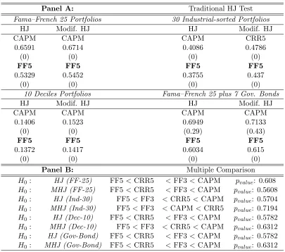
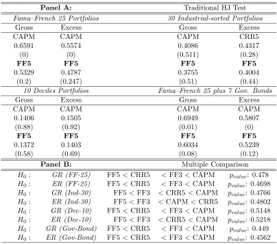
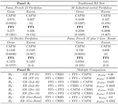
(21) Chapter 1. Comparing Asset Pricing Models: What does the Hansen–Jagannathan Distance Tell Us? 10 From Table 1.1 to Table 1.3, we have ranked candidates in terms of the HJ, the modified, the unconstrained, and the constrained HJ distance measures. In every test portfolios section, the first row shows that model which obtains the largest normalized pricing errors; the second row gives the least misspecified (the one that gets the smallest normalized pricing errors). All distance measures are first tested by the null hypothesis that the HJ distance is equal to zero, and then are tested by the null hypothesis the least misspecified candidate has the smallest normalized pricing errors via block bootstrapping. For gross returns of all test portfolios, the Fama–French five-factor model obtains smaller HJ, modified HJ, unconstrained, and constrained distance measures than the other three models: its normalized pricing errors are the smallest and are robust among different estimating methods compared with the CAPM, the Fama–French three-factor, and the Chen, Roll, and Ross five-factor. On the other hand, the CAPM has the largest normalized pricing errors among the three sample test portfolios. Here, through the multiple comparison test, we cannot statistically reject the null hypothesis that the Fama–French five-factor has the smallest distance measure. While explaining excess returns on assets, the Fama–French five-factor performs better than others again, but the Chen, Roll, and Ross five-factor macro model is not able to capture the industry effect (it is even worse than the traditional CAPM). Interestingly, the traditional HJ distance test is misleading in this case. For instance, the least and the most misspecified ones both have p-values larger than 5% for the test. This means that we cannot statistically reject the null hypothesis that both of their HJ distance measures are zero. However, after implementing multiple comparison tests, all bootstrapping pvalues for the rankings are greater than 0.05: we cannot statistically reject the null hypothesis that the least misspecified model outperforms the others because of their relatively smaller normalized pricing errors. Overall, the Fama–French five-factor model performs best in terms of the normalized pricing errors, compared with the other candidates. The result maintains among the four HJ distance measures. On the other hand, the traditional CAPM cannot successfully prices payoffs on cross-section assets; the macro-factor model, the Chen, Roll, and Ross five-factor, is not able to explain industry portfolios: its performance is even worse than CAPM.. 1.4.3. Empirical Results on Consumption-Based Models. The consumption-based CAPM has been criticized by the literature for the low correlation between the consumption growth and equity returns. In this part, we treat the.

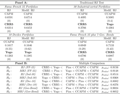
(22) Chapter 1. Comparing Asset Pricing Models: What does the Hansen–Jagannathan Distance Tell Us? 11 consumption-based CAPM as the benchmark model. The Chen, Roll, and Ross fivefactor macro model is also included in order to compare a pure macro-factor model with macro-derived models (the Yogo non-durable and durable consumption and the Piazzesi, Schneider, and Tuzel housing consumption model). According to tables from 1.4 to 1.6, the Chen, Roll, and Ross macro-factor model statistically dominates the others, getting the smallest normalized pricing errors when explaining payoffs on the 25 Fama–French size–value and the yields on U.S. government bonds; the consumption-based CAPM is able to explain these two portfolios better than the CAPM. The Yogo non-durable and durable model outperforms the others in capturing the industry and size effects, except for the case when the Chen, Roll, and Ross five-factor model performs well in pricing the gross returns on 30 industry portfolios in terms of the traditional HJ distance. On the other hand, the consumption-based CAPM is not able to capture these effects, and even the CAPM performs relatively better. Again, rather than testing whether the HJ distance is equal to zero, we show that all p-values on multiple comparisons tests are statistically larger than 5%, therefore we cannot reject the null hypothesis that the Chen, Roll, and Ross five-factor, and the Yogo models have the smallest pricing errors, compared to the others when explaining excess and gross returns on specific assets. Overall, the Chen, Roll and Ross macro-factor model outperforms others to explain returns on 25 Fama–French size-value stocks and yields on U.S. government bonds; the consumption-based CAPM outperforms the CAPM. Moreover, the Yogo non-durable and durable consumption model is the least misspecified model to capture industry and size effects.. 1.4.4. Empirical Results on Scaled Consumption-Based Models. Here, the consumption-based CAPM and Chen, Roll and Ross macro-factor model are chosen as the benchmark. From Table 1.7 to 1.9, all conditional C-CAPMs outperform the C-CAPM in explaining cross sectional payoffs, except for the Santos and Veronesi scaled C-CAPM with labor income in pricing payoffs to size portfolios. In particular, in explaining payoffs on 25 Fama–French size–value portfolios, the Chen, Roll and Ross macro-factor model has smaller normalized pricing errors than the others in terms of the unconstrained and the constrained HJ distance measures; the Santos and Veronesi conditional C-CAPM can perform well in pricing gross returns on 25 Fama–French size–value portfolios in terms.

(23) Chapter 1. Comparing Asset Pricing Models: What does the Hansen–Jagannathan Distance Tell Us? 12 of the HJ distance, and the scaled housing consumption-based model is able to explain excess returns well in terms of the modified HJ distance. While capturing the industry effect, the Lettau and Ludvigson conditional CAPM obtains the smallest normalized pricing errors; the labor income scaled C-CAPM outperforms others in pricing its excess returns. On the other hand, the labor income scaled C-CAPM fails to explain the size effect, while the Lettau and Ludvigson conditional CCAPM dominates others in getting the smallest pricing errors. A special case happens when the Chen, Roll, and Ross five-factor model is used to price gross returns on size portfolios: it performs best. In U.S. government bond portfolios, the labor income scaled C-CAPM outperforms the others in explaining gross yields, while the scaled housing consumption and the macrofactor models are outstanding in explaining net yields in terms of the modified and the unconstrained HJ distance measures, respectively. Overall, the pricing performances on conditional models is unstable, meanwhile the Chen, Roll and Ross macro-factor model outperforms to explain size–value stocks, gross returns on size portfolios and net yields on U.S. government bond portfolios. Through the multiple comparison test, the chosen models are the least misspecified ones to explain specific test portfolios.. 1.4.5. Economic Interpretations. When all models are misspecified, the HJ distance measure gives the statistic criteria on the normalized pricing errors to explain asset returns. In this section, we have analyzed the economic reasons that why those models outperform others to explain specific test portfolios. For most return-based models, factors are obtained directly from the financial market. For instance, size and book-to-market ratio factors are well-known to explain Fama– French size-value portfolios, hence, Fama and French three- and five- factors explain more than 90% of the time-series variation in portfolios’ returns and more than 75% of the cross-sectional variation in their average returns. Given those features, it is reasonable for the Fama–French factor model to obtain a relative low value of HJ distance, because it is likely to produce betas that line up with expected returns; given the test portfolios, the Fama–French factor residuals of the size-value portfolios is tiny. For consumption-based asset pricing models, the intuition on a ‘successful’ consumption factor is different from using financial factors to explain equity returns. Small stocks and value stocks deliver relatively low returns during recessions, which explain their high.

(24) Chapter 1. Comparing Asset Pricing Models: What does the Hansen–Jagannathan Distance Tell Us? 13 average returns relative to big stocks and growth stocks. When utility is nonseparable in non-durable and durable consumption (or housing consumption) and the elasticity of substitution between the two consumption goods is sufficiently high, marginal utility rises when durable consumption (or housing consumption) falls. Therefore stock returns are unexpectedly low at business cycle troughs, when durable consumption (or housing consumption) falls sharply, which explain the cross-sectional variation and the countercyclical variation in the equity premium. There is a little data difference between durable consumption in Yogo (2006) and housing consumption in Piazzesi et al. (2007): NIPA provides a direct measure of service flow for real estate, whereas it only reports expenditure on other durables. For the conditional consumption-based models, the fact that scaled factor models have smaller HJ distances than non-scaled factor models comes from two sources. Mainly, the conditioning information reduces the pricing errors by allowing the prices of risks to vary with the business cycle. Then, by doubling the number of parameters, a scaled factor model uses additional degrees of freedom in the minimization problem and is better able to fit the data. This better fit may be spurious, though, as small sample biases may worsen. Another important issue is the stability of the model’s parameters. If the conditional version is correctly specified and captures the dynamics in risk premiums, it will outperform the unconditional model. However, if the implied time-varying risk premiums are inherently misspecified because we choose the wrong conditioning variable, this false model may still appear to work well in small samples since it uses additional degrees of freedom. Ghysels (1998) finds that conditional models are fragile and may have bigger pricing errors than unconditional models. How to compare the conditional asset pricing models is worthy to investigating in future research.. 1.5. Conclusions. Multi-factor linear asset pricing models play an important role in evaluating portfolio performances and cost-of-capital applications for practitioners. In this paper, we apply various HJ distance measures to understand which linear factor model outperforms to explain cross-sectional financial assets, and to seek an economic interpretation of the specifications that appears most promising. We find that the Fama–French five-factor is ranked top in terms of misspecified measures in explaining the Fama–French size-value and these equities combined with seven government bond portfolios. When pricing returns on industrial-sorted assets, the Yogo durable consumption model performs better than other consumption-based models. For.

(25) Chapter 1. Comparing Asset Pricing Models: What does the Hansen–Jagannathan Distance Tell Us? 14 the conditional consumption-based models, the Lettau and Ludvigson (2001) outperforms others in explaining the gross returns on size portfolios, and Santos and Veronesi conditional CAPM with labor income behaves better to explain the excess returns. Through a multiple comparison test, we show all rankings maintain among gross and excess returns in terms of several distance measures. At last, we explain the economic reason why some models are least misspecified. Moreover, the SDFs of those least misspecified candidates are quite volatile and have clear financial market cycle patterns: some of them capture the periods of financial market crashes. The paper also empirically investigates conditional asset pricing models while scaling risk factors as ‘conditioning down’ the dynamic pricing equation as (1.1). As Cochrane (2001) [26] emphasizes, the conditioning information of economic agents may not be observable, and one cannot omit it in making inferences about the behavior of conditional moments. There are two solutions. One is to identify the conditional Euler equation, but the identification of the conditional mean in the Euler equation requires knowing the joint distribution of mt+1 and the set of test asset returns Rt+1 . Scaling factors is one way to incorporate conditioning information into the pricing kernel. Lettau and Ludvigson (2001) [10] therefore used the terms “scaling” and “conditioning” interchangeably when referring to models with scaled factors even though the models were estimated and tested on unconditional Euler equation moments. An unfortunate consequence may have been to create the case that scaled factor models for the conditional asset pricing models may have been mis-impression, since the conditional beta is always derived from conditional Euler equation moments (scaling returns), whether or not the pricing kernel includes scaled factors. We will work on this topic in future research..

(26) Chapter 1. Comparing Asset Pricing Models: What does the Hansen–Jagannathan Distance Tell Us? 15 Table 1.1: Return-based Models via HJ and Modified HJ Distance Notes: The table reports the Hansen–Jagannathan (HJ) distance, modified HJ distance measures and their tests. In Panel A, HJ distance measures and the traditional HJ test are shown. In every test portfolios section, the third row shows that model which obtains the largest normalized pricing errors; the sixth row gives the least misspecified (the one that gets the smallest normalized pricing errors). All distance measures are tested by the null hypothesis that the HJ distance is equal to zero, the p-values are reported below the distance measure, respectively. In Panel B, multiple comparison for all models are reported. The null hypothesis that the least misspecified one has the smallest distance measure is tested via block-bootstrapping 5000 times.. Panel A: Fama–French 25 Portfolios Modif. HJ HJ CAPM CAPM 0.6591 0.6714 (0) (0) FF5 FF5 0.5329 0.5452 (0) (0) 10 Deciles Portfolios Modif. HJ HJ CAPM CAPM 0.1406 0.1523 (0) (0) FF5 FF5 0.1372 0.1417 (0) (0) Panel B: H0 : HJ (FF-25) H0 : MHJ (FF-25) H0 : HJ (Ind-30) H0 : MHJ (Ind-30) H0 : HJ (Dec-10) H0 : MHJ (Dec-10) H0 : HJ (Gov-Bond) H0 : MHJ (Gov-Bond). FF5 < CRR5 FF5 < CRR5 FF5 < FF3 FF5 < FF3 FF5 < CRR5 FF5 < FF3 FF5 < CRR5 FF5 < CRR5. Traditional HJ Test 30 Industrial-sorted Portfolios HJ Modif. HJ CAPM CRR5 0.4086 0.4786 (0) (0) FF5 FF5 0.3755 0.437 (0) (0) Fama–French 25 plus 7 Gov. Bonds HJ Modif. HJ CAPM CAPM 0.6949 0.7133 (0.29) (0.43) FF5 FF5 0.6034 0.615 (0) (0) Multiple Comparison < FF3 < CAPM pvalue : 0.608 < FF3 < CAPM pvalue : 0.5608 < CRR5 < CAPM pvalue : 0.5704 < CAPM < CRR5 pvalue : 0.7194 < FF3 < CAPM pvalue : 0.5782 < CRR5 < CAPM pvalue : 0.6312 < FF3 < CAPM pvalue : 0.5782 < FF3 < CAPM pvalue : 0.6312.

(27) Chapter 1. Comparing Asset Pricing Models: What does the Hansen–Jagannathan Distance Tell Us? 16. Table 1.2: Return-based Models via Unconstrained HJ Distance Notes: The table reports the unconstrained Hansen–Jagannathan (HJ) distance measure and its test for both gross and excess returns. In Panel A, HJ distance measures and the traditional HJ test are shown. In every test portfolios section, the third row shows that model which obtains the largest normalized pricing errors; the sixth row gives the least misspecified (the one that gets the smallest normalized pricing errors). All distance measures are tested by the null hypothesis that the HJ distance is equal to zero, the p-values are reported below the distance measure, respectively. In Panel B, multiple comparison for all models are reported. The null hypothesis that the least misspecified one has the smallest distance measure is tested via block-bootstrapping 5000 times.. Panel A: Fama–French 25 Portfolios Excess Gross CAPM CAPM 0.6591 0.5574 (0) (0) FF5 FF5 0.5329 0.4787 (0.2) (0.247) 10 Deciles Portfolios Excess Gross CAPM CAPM 0.1406 0.1505 (0.88) (0.92) FF5 FF5 0.1372 0.1403 (0.58) (0.69) Panel B: H0 : GR (FF-25) H0 : ER (FF-25) H0 : GR (Ind-30) H0 : ER (Ind-30) H0 : GR (Dec-10) H0 : ER (Dec-10) H0 : GR (Gov-Bond) H0 : ER (Gov-Bond). FF5 < CRR5 FF5 < CRR5 FF5 < FF3 FF5 < FF3 FF5 < CRR5 FF5 < FF3 FF5 < CRR5 FF5 < CRR5. Traditional HJ Test 30 Industrial-sorted Portfolios Gross Excess CAPM CRR5 0.4086 0.4317 (0.511) (0.28) FF5 FF5 0.3755 0.4004 (0.51) (0.44) Fama–French 25 plus 7 Gov. Bonds Gross Excess CAPM CAPM 0.6949 0.5807 (0.01) (0) FF5 FF5 0.6034 0.5239 (0.08) (0.12) Multiple Comparison < FF3 < CAPM pvalue : 0.478 < FF3 < CAPM pvalue : 0.4698 < CRR5 < CAPM pvalue : 0.4766 < CAPM < CRR5 pvalue : 0.4802 < FF3 < CAPM pvalue : 0.5148 < CRR5 < CAPM pvalue : 0.5218 < FF3 < CAPM pvalue : 0.449 < FF3 < CAPM pvalue : 0.4562.

(28) Chapter 1. Comparing Asset Pricing Models: What does the Hansen–Jagannathan Distance Tell Us? 17. Table 1.3: Return-based Models via Constrained HJ Distance Notes: The table reports the constrained Hansen–Jagannathan (HJ) distance measure and its test for both gross and excess returns. In Panel A, HJ distance measures and the traditional HJ test are shown. In every test portfolios section, the third row shows that model which obtains the largest normalized pricing errors; the sixth row gives the least misspecified (the one that gets the smallest normalized pricing errors). All distance measures are tested by the null hypothesis that the HJ distance is equal to zero, the p-values are reported below the distance measure, respectively. In Panel B, multiple comparison for all models are reported. The null hypothesis that the least misspecified one has the smallest distance measure is tested via block-bootstrapping 5000 times.. Panel A: Fama–French 25 Portfolios Excess Gross CAPM CAPM 0.674 0.607 (0.0324) (0) FF5 FF5 0.577 0.506 (0.1261) (0.134) 10 Deciles Portfolios Excess Gross CAPM CAPM 0.1448 0.1505 (0.6036) (0.567) FF5 FF5 0.1372 0.1407 (0.5757) (0.4) Panel B: H0 : GR (FF-25) H0 : ER (FF-25) H0 : GR (Ind-30) H0 : ER (Ind-30) H0 : GR (Dec-10) H0 : ER (Dec-10) H0 : GR (Gov-Bond) H0 : ER (Gov-Bond). FF5 < CRR5 FF5 < CRR5 FF5 < FF3 FF5 < FF3 FF5 < FF3 FF5 < FF3 FF5 < CRR5 FF5 < CRR5. Traditional HJ Test 30 Industrial-sorted Portfolios Gross Excess CAPM CAPM 0.4109 0.447 (0.5207) (0.476) FF5 FF5 0.3769 0.3896 (0.5593) (0.467) Fama–French 25 plus 7 Gov. Bonds Gross Excess CAPM CAPM 0.726 0.698 (0.0658) (0) FF5 FF5 0.6504 0.61 (0.105) (0.2) Multiple Comparison < FF3 < CAPM pvalue : 0.36 < FF3 < CAPM pvalue : 0.4698 < CRR5 < CAPM pvalue : 0.625 < CRR5 < CAPM pvalue : 0.4802 < CAPM < CRR5 pvalue : 0.63 < CAPM < CRR5 pvalue : 0.5218 < FF3 < CAPM pvalue : 0.6 < FF3 < CAPM pvalue : 0.4562.

(29) Chapter 1. Comparing Asset Pricing Models: What does the Hansen–Jagannathan Distance Tell Us? 18. Table 1.4: Consumption-based Models via HJ and Mod. HJ Distance Notes: The table reports the Hansen–Jagannathan (HJ) distance, modified HJ distance measures and their tests on consumption-based asset pricing models. In Panel A, HJ distance measures and the traditional HJ test are shown. In every test portfolios section, the third row shows that model which obtains the largest normalized pricing errors; the sixth row gives the least misspecified (the one that gets the smallest normalized pricing errors). All distance measures are tested by the null hypothesis that the HJ distance is equal to zero, the p-values are reported below the distance measure, respectively. In Panel B, multiple comparison for all models are reported. The null hypothesis that the least misspecified one has the smallest distance measure is tested via block-bootstrapping 5000 times. Panel A: Fama–French 25 Portfolios Modif. HJ HJ CAPM CAPM 0.6591 0.6714 (0) (0) CRR5 CRR5 0.6314 0.6453 (0) (0) 10 Deciles Portfolios HJ Modif. HJ CCAPM CCAPM 0.1617 0.1646 (0.55) (0.62) Yogo Yogo 0.1263 0.1385 (0) (0) Panel B: H0 : HJ (FF-25) H0 : MHJ (FF-25) H0 : HJ (Ind-30) H0 : MHJ (Ind-30) H0 : HJ (Dec-10) H0 : MHJ (Dec-10) H0 : HJ (Gov-Bond) H0 : MHJ (Gov-Bond). CRR5 < Yogo CRR5 < Piza CRR5 < Yogo Yogo < CRR5 Yogo < CRR5 Yogo < CRR5 CRR5 < Yogo CRR5 < Yogo. < < < < < < < <. Traditional HJ Test 30 Industrial-sorted Portfolios HJ Modif. HJ CCAPM CCAPM 0.4095 0.5085 (0) (0.4) CRR5 Yogo 0.3766 0.4364 (0) (0) Fama–French 25 plus 7 Gov. Bonds HJ Modif. HJ CAPM CAPM 0.6949 0.7133 (0.29) (0.43) CRR5 CRR5 0.6706 0.6887 (0) (0) Multiple Comparison Piza < CCAPM < CAPM pvalue : 0.9156 Yogo < CCAPM < CAPM pvalue : 0.9148 Piza < CAPM < CCAPM pvalue : 0.8514 CAPM < Piza < CCAPM pvalue : 0.9368 CAPM < Piza < CCAPM pvalue : 0.8082 CAPM < Piza < CCAPM pvalue : 0.8376 Piza < CCAPM < CAPM pvalue : 0.9024 Piza < CCAPM < CAPM pvalue : 0.9052.

(30) Chapter 1. Comparing Asset Pricing Models: What does the Hansen–Jagannathan Distance Tell Us? 19. Table 1.5: Consumption-based Models via Unconstrained HJ Distance Notes: The table reports the unconstrained Hansen–Jagannathan (HJ) distance measure and its test for both gross and excess returns for consumption-based asset pricing models. In Panel A, HJ distance measures and the traditional HJ test are shown. In every test portfolios section, the third row shows that model which obtains the largest normalized pricing errors; the sixth row gives the least misspecified (the one that gets the smallest normalized pricing errors). All distance measures are tested by the null hypothesis that the HJ distance is equal to zero, the p-values are reported below the distance measure, respectively. In Panel B, multiple comparison for all models are reported. The null hypothesis that the least misspecified one has the smallest distance measure is tested via block-bootstrapping 5000 times. Panel A: Fama–French 25 Portfolios Excess Gross CAPM CAPM 0.6591 0.5574 (0) (0) CRR5 CRR5 0.5554 0.4944 (0.29) (0.32) 10 Deciles Portfolios Gross Excess CCAPM CCAPM 0.1617 0.1624 (0.81) (0.94) Yogo Yogo 0.1263 0.1372 (0.79) (0.88) Panel B: H0 : GR (FF-25) H0 : ER (FF-25) H0 : GR (Ind-30) H0 : ER (Ind-30) H0 : GR (Dec-10) H0 : ER (Dec-10) H0 : GR (Gov-Bond) H0 : ER (Gov-Bond). CRR5 < Yogo CRR5 < Piza Yogo < CRR5 Yogo < CAPM Yogo < CRR5 Yogo < CRR5 CRR5 < Yogo CRR5 < Yogo. < < < < < < < <. Traditional HJ Test 30 Industrial-sorted Portfolios Gross Excess CCAPM CCAPM 0.4095 0.4533 (0.522) (0.23) Yogo Yogo 0.3957 0.3999 (0.606) (0.66) Fama–French 25 plus 7 Gov. Bonds Gross Excess CAPM CAPM 0.6949 0.5807 (0.01) (0) CRR5 CRR5 0.6294 0.5416 (0.07) (0.1) Multiple Comparison Piza < CCAPM < CAPM pvalue : 0.4412 Yogo < CCAPM < CAPM pvalue : 0.299 Piza < CAPM < CCAPM pvalue : 0.6554 CRR5 < Piza < CCAPM pvalue : 0.7358 CAPM < Piza < CCAPM pvalue : 0.7486 CAPM < Piza < CCAPM pvalue : 0.749 Piza < CCAPM < CAPM pvalue : 0.5018 Piza < CCAPM < CAPM pvalue : 0.3706.

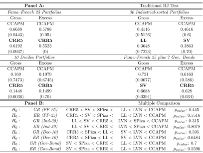
(31) Chapter 1. Comparing Asset Pricing Models: What does the Hansen–Jagannathan Distance Tell Us? 20. Table 1.6: Consumption-based Models via Constrained HJ Distance Notes: The table reports the constrained Hansen–Jagannathan (HJ) distance measure and its test for both gross and excess returns for consumption-based asset pricing models. In Panel A, HJ distance measures and the traditional HJ test are shown. In every test portfolios section, the third row shows that model which obtains the largest normalized pricing errors; the sixth row gives the least misspecified (the one that gets the smallest normalized pricing errors). All distance measures are tested by the null hypothesis that the HJ distance is equal to zero, the p-values are reported below the distance measure, respectively. In Panel B, multiple comparison for all models are reported. The null hypothesis that the least misspecified one has the smallest distance measure is tested via block-bootstrapping 5000 times. Panel A: Fama–French 25 Portfolios Excess Gross CAPM CAPM 0.674 0.56 (0.0324) (0.04) CRR5 CRR5 0.6192 0.54 (0.0937) (0.0708) 10 Deciles Portfolios Gross Excess CAPM CCAPM 0.169 0.56 (0.7473) (0.045) Yogo Yogo 0.128 0.1376 (0.8) (0.3) Panel B: H0 : GR (FF-25) H0 : ER (FF-25) H0 : GR (Ind-30) H0 : ER (Ind-30) H0 : GR (Dec-10) H0 : ER (Dec-10) H0 : GR (Gov-Bond) H0 : ER (Gov-Bond). CRR5 < Yogo CRR5 < Yogo Yogo < CRR5 Yogo < CRR5 Yogo < CAPM Yogo < CAPM CRR5 < Yogo CRR5 < Yogo. < < < < < < < <. Traditional HJ Test 30 Industrial-sorted Portfolios Gross Excess CCAPM CCAPM 0.4116 0.467 (0.5126) (0.678) Yogo Yogo 0.3984 0.405 (0.5853) (0.593) Fama–French 25 plus 7 Gov. Bonds Gross Excess CAPM CCAPM 0.726 0.467 (0.0658) (0.04) CRR5 CRR5 0.684 0.62 (0.0687) (0.051) Multiple Comparison Piza < CCAPM < CAPM pvalue : 0.545 Piza < CCAPM < CAPM pvalue : 0.299 Piza < CAPM < CCAPM pvalue : 0.64 Piza < CAPM < CCAPM pvalue : 0.7358 CRR5 < Piza < CCAPM pvalue : 0.75 CRR5 < Piza < CCAPM pvalue : 0.749 Piza < CCAPM < CAPM pvalue : 0.5 Piza < CCAPM < CAPM pvalue : 0.3706.

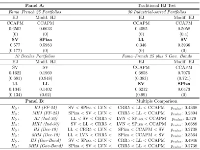
(32) Chapter 1. Comparing Asset Pricing Models: What does the Hansen–Jagannathan Distance Tell Us? 21. Table 1.7: Cond. Consumption-based Models via HJ and Mod. HJ Dist. Notes: The table reports the Hansen–Jagannathan (HJ) distance, modified HJ distance measures and their tests on conditional consumption-based asset pricing models. In Panel A, HJ distance measures and the traditional HJ test are shown. In every test portfolios section, the third row shows that model which obtains the largest normalized pricing errors; the sixth row gives the least misspecified (the one that gets the smallest normalized pricing errors). All distance measures are tested by the null hypothesis that the HJ distance is equal to zero, the p-values are reported below the distance measure, respectively. In Panel B, multiple comparison for all models are reported. The null hypothesis that the least misspecified one has the smallest distance measure is tested via block-bootstrapping 5000 times. Panel A: Fama–French 25 Portfolios HJ Modif. HJ CCAPM CCAPM 0.6502 0.6623 (0) (0) SV SPiza 0.577 0.5983 (0.177) (0) 10 Deciles Portfolios HJ Modif. HJ SV SV 0.1622 0.1969 (0.681) (0.948) LL LL 0.1345 0.1402 (0.134) (0.02) Panel B: H0 : HJ (FF-25) H0 : MHJ (FF-25) H0 : HJ (Ind-30) H0 : MHJ (Ind-30) H0 : HJ (Dec-10) H0 : MHJ (Dec-10) H0 : HJ (Gov-Bond) H0 : MHJ (Gov-Bond). SV < SPiza < LVN SPiza < SV < LVN LL < SV < CRR5 SV < LL < CRR5 LL < CRR5 < LVN LL < LVN < CRR5 SV < SPiza < LVN SPiza < SV < LVN. < < < < < < < <. Traditional HJ Test 30 Industrial-sorted Portfolios HJ Modif. HJ CCAPM CCAPM 0.4095 0.5058 (0) (0.4) LL SV 0.346 0.3936 (0) (0) Fama–French 25 plus 7 Gov. Bonds HJ Modif. HJ CCAPM CCAPM 0.6858 0.7075 (0.383) (0.721) SV SPiza 0.6212 0.6473 (0.99) (0) Multiple Comparison CRR5 < LL < CCAPM pvalue : 0.4368 CRR5 < LL < CCAPM pvalue : 0.2394 LVN < SPiza < CCAPM pvalue : 0.379 LVN < SPiza < CCAPM pvalue : 0.6688 SPiza < CCAPM < SV pvalue : 0.2738 SPiza < CCAPM < SV pvalue : 0.3564 CRR5 < LL < CCAPM pvalue : 0.4946 CRR5 < LL < CCAPM pvalue : 0.2738.

(33) Chapter 1. Comparing Asset Pricing Models: What does the Hansen–Jagannathan Distance Tell Us? 22. Table 1.8: Cond. Consumption-based Models via Unconst. HJ Dist. Notes: The table reports the unconstrained Hansen–Jagannathan (HJ) distance measure and its test for both gross and excess returns for conditional consumption-based asset pricing models. In Panel A, HJ distance measures and the traditional HJ test are shown. In every test portfolios section, the third row shows that model which obtains the largest normalized pricing errors; the sixth row gives the least misspecified (the one that gets the smallest normalized pricing errors). All distance measures are tested by the null hypothesis that the HJ distance is equal to zero, the p-values are reported below the distance measure, respectively. In Panel B, multiple comparison for all models are reported. The null hypothesis that the least misspecified one has the smallest distance measure is tested via block-bootstrapping 5000 times. Panel A: Fama–French 25 Portfolios Gross Excess CCAPM CCAPM 0.6502 0.5522 (0.014) (0) CRR5 CRR5 0.5554 0.4944 (0.2926) (0.315) 10 Deciles Portfolios Gross Excess SV SV 0.1622 0.1932 (0.483) (0.7) LL LL 0.1345 0.1388 (0.87) (0.94) Panel B: H0 : GR (FF-25) H0 : ER (FF-25) H0 : GR (Ind-30) H0 : ER (Ind-30) H0 : GR (Dec-10) H0 : ER (Dec-10) H0 : GR (Gov-Bond) H0 : ER (Gov-Bond). CRR5 < SV < SPiza CRR5 < SPiza < SV LL < SV < CRR5 SV < LL < CRR5 LL < CRR5 < LVN LL < LVN < CRR5 SV < SPiza < CRR5 CRR5 < SPiza < SV. < < < < < < < <. Traditional HJ Test 30 Industrial-sorted Portfolios Gross Excess CCAPM CCAPM 0.4095 0.4533 (0.522) (0.23) LL SV 0.346 0.3663 (0.851) (0.856) Fama–French 25 plus 7 Gov. Bonds Gross Excess CCAPM CCAPM 0.6858 0.5776 (0.02) (0.01) SV CRR5 0.6212 0.5416 (0.05) (0.1) Multiple Comparison LVN < LL < CCAPM pvalue : 0.5434 LVN < LL < CCAPM pvalue : 0.5516 LVN < SPiza < CCAPM pvalue : 0.3982 LVN < SPiza < CCAPM pvalue : 0.8678 SPiza < CCAPM < SV pvalue : 0.4624 SPiza < CCAPM < SV pvalue : 0.6484 LVN < LL < CCAPM pvalue : 0.7398 LVN < LL < CCAPM pvalue : 0.5596.

(34) Chapter 1. Comparing Asset Pricing Models: What does the Hansen–Jagannathan Distance Tell Us? 23. Table 1.9: Cond. Consumption-based models via Constrained HJ Dist. Notes: The table reports the constrained Hansen–Jagannathan (HJ) distance measure and its test for both gross and excess returns for conditional consumption-based asset pricing models. In Panel A, HJ distance measures and the traditional HJ test are shown. In every test portfolios section, the third row shows that model which obtains the largest normalized pricing errors; the sixth row gives the least misspecified (the one that gets the smallest normalized pricing errors). All distance measures are tested by the null hypothesis that the HJ distance is equal to zero, the p-values are reported below the distance measure, respectively. In Panel B, multiple comparison for all models are reported. The null hypothesis that the least misspecified one has the smallest distance measure is tested via block-bootstrapping 5000 times. Panel A: Fama–French 25 Portfolios Gross Excess CCAPM CCAPM 0.6688 0.5788 (0.0443) (0.05) CRR5 CRR5 0.6192 0.5523 (0.0937) (0) 10 Deciles Portfolios Gross Excess CCAPM CCAPM 0.169 0.1979 (0.7473) (0.6745) CRR5 CRR5 0.1448 0.1499 (0.6036) (0.70) Panel B: H0 : GR (FF-25) H0 : ER (FF-25) H0 : GR (Ind-30) H0 : ER (Ind-30) H0 : GR (Dec-10) H0 : ER (Dec-10) H0 : GR (Gov-Bond) H0 : ER (Gov-Bond). CRR5 < SV < SPiza CRR5 < SV < SPiza LL < SV < CRR5 LL < SV < CRR5 CRR5 < SPiza < LL CRR5 < SPiza < LL SV < SPiza < CRR5 SV < SPiza < CRR5. < < < < < < < <. Traditional HJ Test 30 Industrial-sorted Portfolios Gross Excess CCAPM CCAPM 0.4116 0.4616 (0.5126) (0.6) LL SV 0.3648 0.3863 (0.7223) (0.70) Fama–French 25 plus 7 Gov. Bonds Gross Excess CCAPM CCAPM 0.721 0.6163 (0.0677) (0.586) SV CRR5 0.6688 0.628 (0.0394) (0.034) Multiple Comparison LL < LVN < CCAPM pvalue : 0.445 LL < LVN < CCAPM pvalue : 0.5516 LVN < SPiza < CCAPM pvalue : 0.315 LVN < SPiza < CCAPM pvalue : 0.8678 SV < LVN < CCAPM pvalue : 0.595 SV < LVN < CCAPM pvalue : 0.6484 LL < LVN < CCAPM pvalue : 0.7 LL < LVN < CCAPM pvalue : 0.5596.

(35) Chapter 1. Comparing Asset Pricing Models: What does the Hansen–Jagannathan Distance Tell Us? 24. Figure 1.1: Hansen–Jagannathan Distance Notes: Figure shows that the Hasen–Jagannathan (HJ) distance is the least squared distance between any point along the admissible SDF line and the cross point between these two orthogonal lines (the payoffs line). Here it assumes that there are only two states on nature, then the payoffs line is a combination of the payoff on each state. The circle point is the proposed stochastic discount factor (SDF), the purple line denotes the HJ (unconstrained) distance and the blue dash line shows the constrained HJ distance..

(36) Chapter 2. Leisure, Consumption and Long Run Risk: An Empirical Evaluation 2.1. Introduction. This paper investigates the ability of a long-run risks asset pricing model, with nonseparable leisure and consumption, to explain the cross-section of asset returns. Using two long-run factors estimated via a VAR, news about future consumption growth and news about leisure, we find that the model does well, relative to other consumptionbased models, in explaining the risk-return profile of size, industry and value-growth portfolios. We build on a rich prior literature starting with Eichenbaum et al. (1988) [6] that explores the empirical properties of intertemporal asset pricing models where the representative agent has utility over consumption and leisure. In this paper we use the framework in Uhlig (2007) [7], which allows for a stochastic discount factor with news about long-run growth in consumption and leisure. An important class of models, introduced by Bansal and Yaron (BY (2005) [27]) rely on long-run consumption growth factors to explain aggregate stock market behavior. The BY model requires a highly persistent consumption process. However, the persistence of such a predictable component in consumption growth is hard to measure in the data. In contrast, leisure data shows more persistence and is correlated with equity returns. As a result introducing non-separable leisure and consumption into the long run model leads to nontrivial interaction between consumption and leisure choice and heightens the volatility of the stochastic discount factor (SDF). 25.

(37) Chapter 2. Leisure, Consumption and Long Run Risk: An Empirical Evaluation. 26. Our paper is related to recent work in Yang (2010) [8]. He defines leisure as the difference between a fixed time endowment and the observable hours spent on working, home production, schooling, communication, and personal care. Our work uses instead adjusted working hours as a measure of leisure. This allows us to avoid misleading results when applying a VAR1 . In other work, Dittmar and Palomino (2010) [29] also investigate the role of labor income risk in the non-separable consumption-leisure model. This paper directly studies the leisure effect in the pricing kernel instead of the long-run relations between real wage, labor and consumption. To evaluate our long-run model, we assess the performance with two measures competing against standard asset pricing models to explain size, industry and value-growth portfolios. Through cross-sectional regressions, we find that the long-run consumption-leisure model cannot be rejected by the J–statistics: it obtains zero pricing errors. Meanwhile the consumption-based CAPM, the Yogo durable consumption and Fama–French three-factor models do not achieve. We also rank the normalized pricing errors by Hansen–Jagannathan (HJ) distance misspecified measures: our model statistically obtains smaller HJ distance than other candidates. Furthermore, we find that the equity premium arises, if assets are highly exposed to long-run consumption risk and long-run leisure risk. Intuitively, while the consumption growth falls, the leisure increases and decreases the price of long-run risks. Hence, compositing high long-run consumption and high long-run leisure with a negative sign, stocks will be asked for more compensation. To empirically test our model, we conduct time-series regressions, and evidence that more risky stocks obtain higher long-run consumption betas and higher negative long-run leisure betas. In the rest of the present paper, we first evidence some stylized facts from the data in Section 2.2. Section 2.3 introduces the basic model and derives the SDF. Section 2.4 specifies the estimation method and describes the data. In Section 2.5, we show the empirical results. Section 2.6 concludes.. 2.2 2.2.1. Stylized Facts Leisure and Consumption. Figure 2.2 shows the average weekly leisure, which takes into account demographic and sectoral movements2 . On average, the amount of leisure is about 44 hours per week 1 Francis and Ramey (2009)[28] point that the demographic effect in working hours gives conflicting results on the effects of technology shocks on working hours via the VAR estimation 2 The activities with the highest enjoyment scores (sex, playing sports, etc.) are those that one would generally classify as leisure (Figure 2.1 shows a survey reported in Robinson and Godbey (1999))..

(38) Chapter 2. Leisure, Consumption and Long Run Risk: An Empirical Evaluation. 27. and strongly counter-cyclical. Non-durable consumption and services is shown in Figure 2.3. Leisure growth exhibits large oscillations during the pre-WWII period, but stays relatively tranquil during the post-war period in Figure 2.4. The leisure growth stays low most of time, but it becomes large occasionally, especially after the financial crisis period of 2007. The volatility of leisure growth is about 27.96% (35.22% and 27.04% for demographic, productivity and Tornqvist adjusted measures). Panel A in Table 2.1 reports the significant first order autocorrelations of leisure as 0.38. As in Bansal and Yaron (2005) [27], the variance ratio test is performed on both its log and realized volatility of innovations. Panel B reports the variance ratio test for leisure. If it is an i.i.d., then the ratio should be equal to 1, but the ratio for leisure is higher than unity implies that a positive autocorrelation dominates. Panel C investigates the time-varying volatility of leisure, since it shows that the adjusted variance ratios are all below unity, which, together with the decreasing variance ratios, provides evidence of a negative serial correlation in the realized volatility. Panel D explores the predictive relations between the realized growth and the price–dividend ratio. The results indicate that realized leisure growth in the future is predicted by the log price–dividend ratio, ∆l,t+j = aj + bj (pt − dt ) + ηt+j ,. (2.1). with negative slopes. Conversely, log price–dividend ratios in the future are also predicted by the realized leisure growth, (pt+j − dt+j ) = aj + bj ∆l,t + ηt+j ,. (2.2). also with negative slopes. Both sets of results are statistically strong. Table 2.2 presents the empirical properties for quarterly per capita nondurable consumption and services. Panel A reports a significant first order autocorrelation of 0.28, which is close to that reported in Bansal and Yaron (2005) [27]. Notably, the autocorrelations for leisure and consumption exhibit patterns that are very similar both qualitatively and quantitatively. Panel B and Panel C show that the short run consumption is close to a random walk, but the volatility is time-varying when the time horizon increases. Panel D provides further evidence for the positive predictive relations between the realized consumption growth and the price–dividend ratio. These results are similar to those reported in Bansal et al. (2005) [30] for nondurable consumption growth..