Facultad de Ciencias Exactas y Naturales
Instituto de F´ısica
Quantum disc plus inverse square potential. An
analytical model for two-dimensional quantum
rings: Study of nonlinear optical properties
by
Carlos Mario Duque Jim´
enez
M.Sc. thesis
Facultad de Ciencias Exactas y Naturales Instituto de F´ısica
Los miembros del Comit´e de postgrado de la Universidad de Antioquia recomendamos que la Tesis “Quantum disc plus inverse square potential. An analytical model for two-dimensional quantum rings: Study of nonlinear optical properties”, realizada por el alumno Carlos Mario Duque Jim´enez, sea aceptada para su defensa como opci´on al grado de Maestr´ıa en F´ısica.
Miguel E. Mora-Ramos Carlos A. Duque
Asesor Revisor
Vo. Bo.
Diego Restrepo Instituto de F´ısica
Contents
1 Introduction 1
2 Preliminaries 3
2.1 Introduction . . . 3
2.2 Density Matrix Equations . . . 3
2.3 Linear And Non-Linear Absorption Coefficients . . . 10
2.4 Linear and Non-Linear Change In The Refractive Index . . . 12
3 A Model For Two-Dimensional Quantum Rings: Optical Properties 14 3.1 Eigenstates And Eigenvalues Of The System . . . 14
3.2 Non-Linear Optics . . . 20
3.3 Results and discussion . . . 22
4 Conclusions 30
Introduction
The confinement of charge carriers in quantum heterostructures through parabolic or semiparabolic potentials has been described in a relatively large number of reports during the two last decades. We can mention here, as examples, some initial works related to the study of electronic, optic and polaronic properties [1, 2, 3, 4, 5] and the calculation of the binding energies of hydrogenic impurities in quantum wells [6]. We can also find more recently works that investigate the specific characteristics of the optical properties in parabolic confined systems [7, 8, 9, 10, 11, 12].
The fabrication of quantum dots (QD) and quantum rings (QR) semiconductors has come true by using self-assembly techniques in crystal growth (see, for example, reference [13]). These two types of systems turn out be of great interest due to the promising prospects of its application in the design and production of optoelectronic devices [14, 15, 16, 17]. Furthermore, going beyond the case of an isolated nanostructure, we have the possibility of producing artificial molecules from QDs or QRs coupling, which becomes a very attractive and promising option in the field of quantum information processing [18], also in the obtention of devices operating in the frequency range of the order of terahertz [19].
By an extension of the classical theory of Balian and Bloch, Tatievski and collaborators [20] have determined the structure of electron shells associated with the motion in closed orbits for mesoscopic systems such as atomic clusters, discs and rings. They have obtained analytical expressions for the density of states in the shell structure, which is a very useful tool to calculate the fluctuations in the binding energies and ionization potentials. Moreover, Tan and Inkson [21] have used an exactly soluble to study the magnetization and the existence of persistent currents of electrons confined in two-dimensional mesoscopic rings and dots, which enables the investigation of these properties over a wide range of devices geometries containing a large number of electrons. They showed that in the limit of weak magnetic field, the persistent current is simply proportional to the magnetization, presenting oscillations of Aharonov-Bohm type. In the same direction, Avishai and Kohmoto have investigated the electronic currents in equilibrium and the magnetization in the case of an ideal two-dimensional disk under the influence of a strong magnetic field [22].
There exists a significant number of research reports related to the linear and nonlinear optical response in QDs with parabolic confinement. To cite only a few examples we mention here the work of the references [23, 24, 25, 26, 27]. Furthermore, there is a particular type of quasi-zero-dimensional system quantum known as quantum disk (QDC) – or shaped disc quantum dot – which has attracted some attention to study this type of optical properties [28, 29, 30, 31, 32]. This is precisely the type of system being studied in this thesis.
We will here dedicate to investigate the electronic states in quantum disks which are under the combined influence of two different types of confinement profiles: one parabolic type and one originating from the action of a potential that depends inversely on the square of the distance. All this is complemented by the presence of an externally applied magnetic field. It must be said that the inverse square potential appeared as a model for the interaction between particles in the quantum problem ofN particles in a parabolic potential and with an additional magnetic field [33]. We will discuss how the inclusion of this kind of potential along with the other two
mentioned fields can serve as a fairly direct model for charge carriers states confined in a two-dimensional semiconductor quantum ring. We will demonstrate that the corresponding electronic eigenstates from the Schr¨odinger like effective mass equation in the conduction band can be obtained analytically. Then, with the use of these states so determined we will calculate the linear and nonlinear contributions to the optical absorption coefficients and relative change of refraction index on a system with the above geometry, based on GaAs. Is appropriate to mention that this issue has attracted significant attention very recently. this is confirmed with the almost simultaneous publication of two original articles in international indexed journals together with our [31, 32].
Preliminaries
2.1 Introduction
The general theory of the nonlinear optical response must be adapted to the situation of low dimen-sional systems in which the spectrum of energy states may have a contribution of discrete energies apart from the continuous states associated with subbands corresponding to free movements with effective mass along one or two dimensions. The situation in which we have a completely discrete spectrum is the quantum dot case, which is analogous to the resulting atomic case. The works of Rosencher and Bois [34] and Ahn and Chuang [35] were those who entered the formalism developed in the 1960 years to the situation of systems as we are concerned.
Now will present a detailed derivation of the first and third-order absorption coefficients as well as the first and thir-order change in the refractive index coefficient in the scheme of reference [35] which was developed for the case of a quantum well. However, the scheme is directly extended to quantum wires and dots.
2.2 Density Matrix Equations
Lets consider a system in the presence of an optical radiation of frequencyωwith polarization along thez-axis. Lets denote ˆρ, ˆH0, ˆM andE(t) as the density matrix for one electron, the unperturbed
Hamiltonian of the system, the electric dipole operator and the intensity of the electric field of the optical radiation of frequencyω respectively.
The density matrix equation for one electron with intraband relaxation is given by
∂ρˆ ∂t =
1
i~[ ˆH0−MˆE(t), ρ]˜ −
1
2[ˆΓ(ˆρ−ρˆ
(0)) + (ˆρ−ρˆ(0))ˆΓ], (2.1)
where ˆρ(0) is the unperturbed density matrix and ˆΓ is a phenomenological operator responsible of
the damping due to electron-phonon, electron-electron and other interaction processes. We assume that ˆΓ is a diagonal matrix and its element Γmm is the inverse of the relaxing time for the estate |m⟩. To simplify the analysis we focus on two-level systems (|1⟩,|2⟩).
The incident monochromatic field is defined as
E(t) = Re(E0e−iωt) =
1 2E0e
−iωt+1
2E0e
iωt= ˜Ee−iωt+ ˜Eeiωt. (2.2)
The diagonal elements of the ˆΓ operator are given by
⟨1|Γˆ|1⟩=γ11= 1/τ1 , ⟨2|Γˆ|2⟩=γ22= 1/τ2. (2.3)
We can solve equation (1) through a perturbative series in ˆρas
ˆ
ρ(t) =∑ n
ˆ
ρ(n)(t). (2.4)
In thermal equilibrium, the density matrix ˆρ(0) is a diagonal matrix where its diagonal elements
are the superficial thermal population. Lets callρ(11n)=⟨1|ρˆ|1⟩,ρ (n)
12 =⟨1|ρˆ|2⟩,ρ (n)
21 =⟨2|ρˆ|1⟩, and
ρ(22n)=⟨2|ρˆ|2⟩. The matrix ˆρhas the hermiticity propertyρ12(t) =ρ∗21(t).
Replacing equation (4) in equation (1), we obtain
∑ n ∂ρˆ ∂t = 1 i~ ∑ n [
( ˆH0−M E(t))ˆˆ ρ(n)−ρˆ(n)( ˆH0−M E(t))ˆ
]
−12∑ n
[ˆΓ(ˆρ(n)−ρˆ(0)) + (ˆρ(n)−ρˆ(0))ˆΓ]. (2.5)
Note that we can write
∑
n ˆ
ρ(n)−ρˆ(0) =∑ n
ˆ
ρ(n+1), (2.6)
then, ∑ n ∂ρˆ ∂t = 1 i~ ∑ n [
( ˆH0−M E(t))ˆˆ ρ(n)−ρˆ(n)( ˆH0−M E(t))ˆ
]
−12 [ ˆ Γ ( ∑ n ˆ ρ(n+1)
) + ( ∑ n ˆ ρ(n+1)
) ˆ Γ ]
. (2.7)
With the last expression we can calculate⟨2|∂∂tρˆ|1⟩, so
∑
n ∂ρ(21n)
∂t = 1 i~ ∑ n [
⟨2|[ ˆH0−M E(t)]ˆˆ ρ(n)|1⟩ − ⟨2|ρˆ(n)[ ˆH0−M E(t)]ˆ |1⟩
]
−12∑ n
[⟨2|Γˆˆρ(n+1)|1⟩+⟨2|ρˆ(n+1)Γˆ|1⟩]. (2.8)
Having present that ˆH0|m⟩=Em|m⟩, we have
∑
n ∂ρ(21n)
∂t = 1 i~ ∑ n [
E2⟨2|ρˆ(n)|1⟩ − ⟨2|Mˆρˆ(n)|1⟩E(t)−E1⟨2|ρˆ(n)|1⟩+⟨2|ρˆ(n)Mˆ|1⟩E(t)
]
−12∑ n
[⟨2|Γˆˆρ(n+1)|1⟩+⟨2|ρˆ(n+1)Γˆ|1⟩]. (2.9)
Introducing the completeness relation given by,
we obtain
∑
n ∂ρ(21n)
∂t = 1 i~ ∑ n [
(E2−E1)ρ21(n)− ⟨2|Mˆ (|1⟩⟨1|+|2⟩⟨2|) ˆρ(n)|1⟩E(t)
+⟨2|ρˆ(n)(|1⟩⟨1|+|2⟩⟨2|) ˆM|1⟩E(t)]−1
2 ∑
n
[⟨2|Γ (ˆ |1⟩⟨1|+|2⟩⟨2|) ˆρ(n+1)|1⟩
+⟨2|ρˆ(n+1)(|1⟩⟨1|+|2⟩⟨2|) ˆΓ|1⟩]. (2.11)
Doing some algebraic steps and remembering that ˆΓ only posses diagonal elements we arrive to
∑
n ∂ρ(21n)
∂t = 1 i~ ∑ n [
(E2−E1)ρ(21n)−(M21ρ(11n)+M22ρ(21n))E(t) + (M11ρ21(n)+M21ρ(22n))E(t)
] −∑ n 1 2 (1 τ2 + 1 τ1 )
ρ(21n+1). (2.12)
Regrouping the order of some terms and settingE21=E2−E1,
∑
n ∂ρ(21n)
∂t = 1 i~ ∑ n [
E21ρ(21n)−(ρ (n) 11 −ρ
(n)
22)M21E(t)−(M22−M11)ρ(21n)E(t)
]
−∑ n
γ12ρ(21n+1), (2.13)
where
γ12=γ21=
1 2 (1 τ1 + 1 τ2 ) . (2.14)
Using the fact thatρ(0)21 =ρ (0)
12 = 0 we have
∑
n
ρ(21n)=
∑
n
ρ(21n+1), (2.15)
which allows us to write
∑
n
∂ρ(21n+1)
∂t =
∑
n [
1
i~E21−γ12
]
ρ(21n+1)−
∑
n 1 i~(ρ
(n) 11 −ρ
(n)
22 )M21E(t)
−∑ n
1
i~(M22−M11)E(t)ρ
(n)
21 . (2.16)
∂ρ(21n+1)
∂t =
[ 1
i~E21−γ12
]
ρ(21n+1)−
1 i~(ρ
(n) 11 −ρ
(n)
22 )M21E(t)
−i1~(M22−M11)E(t)ρ(21n). (2.17)
Following an analogous procedure, we can obtain similar expressions:
∂ρ(12n+1)
∂t =
[1
i~E12−γ21
]
ρ(12n+1)− 1 i~(ρ
(n) 22 −ρ
(n)
11 )M12E(t)
−1
i~(M11−M22)E(t)ρ
(n)
12, (2.18)
and
∂ρ(22n+1)
∂t =−γ22ρ
(n+1) 22 −
1 i~(M21ρ
(n)
12 −M12ρ(21n)) ˜E(t), (2.19)
and also
∂ρ(11n+1)
∂t =−γ11ρ
(n+1) 11 −
1 i~(M12ρ
(n)
21 −M21ρ(12n)) ˜E(t). (2.20)
In the las equations we have that M11 =⟨1|Mˆ|1⟩, M12 = ⟨1|Mˆ|2⟩ , M21 =⟨2|Mˆ|1⟩ and M22 =
⟨2|Mˆ|2⟩. Equations (2.17-2.20) can be solved by writing the density matrix elements in terms of sums proportional to exp(±iωt) and equating terms in both sides of the equations with same temporal dependence. In this calculations we neglect terms that correspond to higher harmonics which correspond to successive absorptions and emissions of photons. We are only interested in the steady state, therefore thenth order perturbative term,ρ(n), is written as
ˆ
ρ(n)(t) = ˆ˜ρ(n)(ω)e−iωt+ ˆρ˜(n)(−ω)eiωt, (2.21)
which is valid for oddn. Whennes even, only DC terms are dominant.
If we setn= 1 en equation (2.21) we have
ˆ
ρ(1)(t) = ˆ˜ρ(1)(ω)e−iωt+ ˆρ˜(1)(−ω)eiωt, (2.22)
and takingn= 0 in (2.17) we have an equation forρ(1)21(t) as,
∂ρ(1)21
∂t = [1
i~E21−γ12
] ρ(1)21 −
1 i~(ρ
(0) 11 −ρ
(0)
22)M21E(t)
−i1~(M22−M11)E(t)ρ(0)21. (2.23)
∂ρ(1)21
∂t = [1
i~E21−γ12
] ρ(1)21 −
1 i~(ρ
(0) 11 −ρ
(0)
22)M21E(t).˜ (2.24)
Therefore we can replace equations (2.2) and (2.22) to solve the last equation. After performing some algebraic steps and equating coefficients of exp(−iωt), we have
−iωρ˜(1)21(ω) = [1
i~E21−γ12
] ˜
ρ(1)21(ω)− 1 i~(ρ
(0) 11 −ρ
(0)
22)M21E,˜ (2.25)
which enables us to obtain ˜ρ(1)ba(ω) so
˜
ρ(1)21(ω) =
˜
EM21(ρ(0)11 −ρ (0) 22)
(E21−~ω−i~γ12)
. (2.26)
Now, our task to calculate the term ˜ρ(3)21(ω). For that purpose we must choosen= 2 in equation (2.17)
∂ρ(3)21
∂t = [1
i~E21−γ12
]
ρ(3)21 −i1~(ρ(2)11 −ρ(2)22)M21E(t)
−i1~(M22−M11)E(t)ρ(2)21. (2.27)
At the same time we taken= 3 in equation (2.21) to get
ρ(3)(t) = ˆ˜ρ(3)(ω)e−iωt+ ˆρ˜(3)(−ω)eiωt. (2.28)
Right now we proceed as before, replacing equations (2.2) and (2.28) in (2.27) and equating terms of exp(−iωt). We also clarify that the termsρ(2)11(t),ρ(2)22(t) andρ(2)21(t) are rectification terms that do not change in time and we can directly replace them by ˜ρ(2)11(0), ˜ρ(2)22(0) and ˜ρ(2)21(0) respectively, therefore
−iωρ˜(3)21(ω) =
[1
i~E21−γ12
] ˜
ρ(3)21(ω)−
1 i~(˜ρ
(2) 11(0)−ρ˜
(2)
22(0))M21E˜
−1
i~(M22−M11) ˜Eρ˜
(2)
21(0). (2.29)
Manipulating this equation allows us to obtain ˜ρ(3)21(ω) as
˜
ρ(3)21(ω) = E˜
(E21−~ω−i~γ12)
[
(˜ρ(2)11(0)−ρ˜(2)22(0))M21+ (M22−M11)˜ρ(2)21(0)
]
. (2.30)
Our target is to find the difference ˜ρ(2)11(0)−ρ˜ (2)
22(0). We must use equations (2.19) and (2.20) to
accomplish this. So,
∂ρ(2)22
∂t =−γ22ρ
(2) 22 −
1 i~(M21ρ
(1)
and
∂ρ(2)11
∂t =−γ11ρ
(2) 11 −
1 i~(M12ρ
(1)
21 −M21ρ(1)12)E(t). (2.32)
Focusing in equation (2.32)and knowing that ρ(2)11 is a rectification term, we have that
∂ρ(2)11 ∂t = 0. We also have to replaceρ(1)21 yρ(1)12 by their steady components, i.e, takingt= 0 in equation (2.22). As well, we take the DC component ofE(t), ˜E, then
0 =−γ11ρ˜(2)11(0)−
˜ E i~
[
M12(˜ρ(1)21(ω) + ˜ρ (1)
21(−ω))−M21(˜ρ(1)12(ω) + ˜ρ (1) 12(−ω))
]
(2.33)
The terms ˜ρ(1)12(ω) and ˜ρ(1)21(−ω) are known as non-resonant terms which can be calculated in the same manner of equation (2.26). They are given by
˜
ρ(1)21(−ω) =
˜
EM21(ρ(0)11 −ρ (0) 22)
(~E21+~ω−i~γab) (2.34)
and
˜
ρ(1)12(ω) =
˜
EM12(ρ(0)11 −ρ (0) 22)
(~E21+~ω+i~γab). (2.35)
As we can see, these last two terms present a dependence of~E21+~ωin their denominators, that
cannot have the possibility of entering in resonance in any time. By this fact, we will neglect them in the rest of our calculations, then
0 =−γ11ρ˜(2)11(0)−
˜ E i~
[
M12ρ˜(1)21(ω)−M21ρ˜(1)12(−ω)
]
. (2.36)
Manipulating this expression we obtain ˜ρ(2)aa(0) as
˜
ρ(2)11(0) = iE˜ γ11~
[
M12ρ˜(1)21(ω)−M21ρ˜(1)12(−ω)
]
. (2.37)
Now, we need to replace ˜ρ(1)21(ω), which is given by (2.26) and ˜ρ (1)
12(−ω) that can be obtained in the
same way as (2.26) or simply replacingω→ −ω in equation (2.35). After replacing the mentioned expressions and doing some mathematical steps we have
˜
ρ(2)11(0) =−
2 ˜E2|M
21|2(ρ(0)11 −ρ (0) 22)γ12
γ11[(E21−~ω)2+ (~γ12)2]
. (2.38)
Following a similar procedure and noting that|M21|2 =|M12|2 andγ12=γ21, we can find ˜ρ(2)22(0)
as
˜ ρ(2)22(0) =
2 ˜E2|M
21|2(ρ(0)11 −ρ (0) 22)γ12
where|M21|2=M21M12.
Finally, using (2.38) and (2.39), we arrive to
˜
ρ(2)11(0)−ρ˜(2)22(0) =−2 ˜E2 ( 1
γ11
+ 1 γ22
)
|M21|2(ρ(0)11 −ρ (0) 22)γ12
[(E21−~ω)2+ (~γ12)2]
. (2.40)
Lets obtain now ˜ρ(2)ba(0). We must use (2.16) with n = 1 and remembering that we are only interested in steady terms. Then
∂ρ(2)ba(0)
∂t =
[1
i~E21−γ12
]
ρ(2)21(0)− 1 i~(ρ
(1) 11(0)−ρ
(1)
22(0))M21E˜
−1
i~(M22−M11) ˜Eρ
(1)
21. (2.41)
Since ∂ρ
(2) 21(0)
∂t = 0 and using (2.22) witht= 0, we obtain
0 = [
1
i~E21−γ12
] ˜ ρ(2)21(0)−
1 i~(˜ρ
(1) 11(ω) + ˜ρ
(1)
11(−ω)−ρ˜ (1) 22(ω)−ρ˜
(1)
22(−ω))M21E˜
−i1~(M22−M11) ˜E(˜ρ(1)21(ω) + ˜ρ (1)
21(−ω)). (2.42)
Continuing with ˜ρ(1)11(ω) from the use of (2.38) and takingn= 0, we have
∂ρ(1)11
∂t =−γ11ρ
(1) 11 −
1 i~(M12ρ
(0)
21 −M21ρ(0)12)E(t), (2.43)
and emphasizing again thatρ(0)21 =ρ(0)12 = 0,
∂ρ(1)11
∂t =−γ11ρ
(1)
11. (2.44)
Once again, using (2.22) and equating terms of exp(−iωt), it is possible to obtain
˜
ρ(1)11(ω)(γ11−iω) = 0, (2.45)
which implies that ˜ρ(1)11(ω) = 0. In the same way ˜ρ(1)11(−ω) = ˜ρ(1)22(ω) = ˜ρ(1)22(−ω) = 0.
With these last results and neglecting the non-resonant term ˜ρ(1)21(−ω) we have
0 = [1
i~E21−γ12
] ˜
ρ(2)21(0)−E˜
i~(M22−M11)˜ρ
(1)
21(ω). (2.46)
Manipulating this expression we obtain ˜ρ(2)ba(0), and replacing (2.26),
˜ ρ(2)21(0) =
˜ E2M
21(M22−M11)(ρ(0)11 −ρ (0) 22)
(E21−i~γ12)(E21−~ω−i~γ12)
Replacing (2.40) and (2.47) in equation (2.30) and performing some mathematical steps we finally arrive to
˜
ρ(3)21(ω) = −
˜ EE˜2M
21(ρ(0)11 −ρ (0) 22)
(E21−~ω−i~γ12)
[
2(1/γ11+ 1/γ22)|M21|
2γ 12
(E21−~ω)2+ (~γ12)2
− (M22−M11)
2
(E21−i~γ12)(E21−~ω−i~γ12)
]
. (2.48)
In the spirit of the last derivations, and using previous results, it is possible to calculate the terms ˜
ρ(3)22(ω) and ˜ρ (3)
11(ω). However, such terms, as is mentioned in the work of Ahn and Chuang [?] are
negligible at the time of evaluating the third order absorption coefficient. These terms are
˜
ρ(3)22(ω) = 2iE˜E˜
2|M 12|2
(~ω+i~γ22)Im
[
(M22−M11)(ρ(0)11 −ρ (0) 22)
(E21−i~γ12)(E21−~ω−i~γ12)
]
(2.49)
and
˜
ρ(3)11(ω) = −
2iE˜E˜2|M 12|2
(~ω+i~γ11)Im
[
(M22−M11)(ρ(0)11 −ρ (0) 22)
(E21−i~γ12)(E21−~ω−i~γ12)
]
. (2.50)
Here, Im denotes imaginary part.
2.3 Linear And Non-Linear Absorption Coefficients
With the results of the last section we can calculate the linear and non-linear absorption coefficients in quantum systems. The electronic polarizationP(t) and the optical susceptibilityχ(t) which arise as consequence of the optical fieldE(t) can be expressed through the dipolar operator ˆM and the density matrix as
P(t) =ϵ0χ(ω) ˜Ee−iωt+ϵ0χ(−ω) ˜Eeiωt=
1
VTr(ˆρMˆ), (2.51)
whereV is the volume of the system,ϵ0is the permittivity of the vacuum and Tr denotes the trace
over the diagonal elements of the matrix ˆρMˆ. The susceptibilityχ is related with the absorption coefficientα(ω) as
α(ω) =ω √ µ
ϵRIm(ϵ0χ(ω)), (2.52)
whereµ is the permeability of the system, ϵR is the real part of the permittivity andχ(ω) is the Fourier component ofχ(t) with dependence exp(−iωt). We can write the polarization as
P(t) = 1 V
[
⟨1|ρˆMˆ|1⟩+⟨2|ρˆMˆ|2⟩]. (2.53)
P(t) = 1 V
∑
n [
ρ(11n)M11+ρ(12n)M21+ρ(21n)M12+ρ(22n)M22
]
. (2.54)
With the aid of (2.21)
P(t) = 1 V
∑
n [
˜
ρ11(n)(ω)M11+ ˜ρ12(n)(ω)M21+ ˜ρ21(n)(ω)M12+ ˜ρ22(n)(ω)M22
] e−iωt
∼(−ω). (2.55)
Choosing n = 1, using (2.51), taking away the non-resonant term, equating terms of e−iωt and remembering that ˜ρ11(1)(ω) = ˜ρ22(1)(ω) = 0, allow us to write
ϵ0χ(1)(ω) ˜E=
1 Vρ˜21
(1)(ω)M
12 (2.56)
Solving forϵ0χ(1)(ω), replacing (2.26), taking its imaginary part and using (2.52), we have,
α(1)(ω) =ω √µ
ϵR |M12|2
V
(ρ(0)11 −ρ(0)22)~γ12
(E21−~ω)2+ (~γ12)2. (2.57)
Definingσv = (ρ(0)11 −ρ (0)
22)/V as the three-dimensional concentration of electrons in the system, we
have
α(1)(ω) =ω √ µ
ϵR
|M12|2σv~γ12
(E21−~ω)2+ (~γ12)2
. (2.58)
Following a similar procedure we can find a third-order expression, we are able to begin with
ϵ0χ(3)(ω) ˜E=
1 V
[ ˜
ρ11(3)(ω)M11+ ˜ρ12(3)(ω)M21+ ˜ρ21(3)(ω)M12+ ˜ρ22(3)(ω)M22
]
. (2.59)
Neglecting the non-resonant term ˜ρab(3)(ω), remembering that, as we said before, the terms ˜
ρaa(3)(ω) and ˜ρbb(3)(ω) just induce a small contribution that we can avoid in our calculations. Solving forϵ0χ(3)(ω), replacing equation (2.48), taking its imaginary part and using (2.52), we can
obtain
α(3)(ω, I) = −ω √µ
ϵRE˜
2
|M12|2σvIm
{
1
(E21−~ω−i~γ12)
[
2γ12(γ11+γ22)|M12|2
γ11γ22[(E21−~ω)2+ (~γ12)2]
− (M22−M11)
2
(E21−i~γ12)(E21−~ω−i~γ12)
]}
. (2.60)
Defining the intensityI of the electromagnetic field through the equation
˜
E2= I 2ϵ0nrc
, (2.61)
α(3)(ω, I) = −ω √µ
ϵR
( I
2ϵ0nrc
)
|M12|2σvIm
{ 1
(E21−~ω−i~γ12)
[ 2γ
12(γ11+γ22)|M12|2
γ11γ22[(E21−~ω)2+ (~γ12)2]
− (M22−M11)
2
(E21−i~γ12)(E21−~ω−i~γ12)
]}
. (2.62)
As a fact of simplicity, lets chooseγ11=γ22, which implies thatγ12=γ11=γ22, so
γ12(γ11+γ22)
γ11γ22
= 2. (2.63)
Taking the imaginary part of equation (2.62) and performing a lengthly algebra leads to a more manageable expression for the third-order absorption coefficient as
α(3)(ω, I) = −ω √µ
ϵR
( I
2ϵ0nrc
)
|M12|2σv~γ12
[(E21−~ω)2+ (~γ12)2]2
[
4|M12|2−(M22−M11) 2(3E2
21−4~ωE21+~2(ω2−γ122 ))
E2
21+ (~γ12)2
]
. (2.64)
With (2.58) and (2.63), the optical absorption coefficient is given by
α(ω, I) =α(1)(ω) +α(3)(ω, I). (2.65)
2.4 Linear and Non-Linear Change In The Refractive
Index
In order to calculate the changes in the refractive index, we follow a procedure which is analogous to the one of the last section. In this time, we start with the fact that the change in the refractive index is related with the optical susceptibility through the equation
∆n(ω) nr = Re
(χ(ω)
2n2
r )
. (2.66)
Using equation (2.56), introducing the previous definitions and taking the real part of the expres-sions, allow us to find an expression for the linear change in the refractive index, therefore
∆n(1)(ω)
nr =
σv|M12|2
2n2
rϵ0
E21−~ω
(E21−~ω)2+ (~γ12)2
. (2.67)
Lets calculate now the third order correction to the change in the refractive index parting from equation (2.59), which after the preliminary considerations, can be written as
χ(3)(ω) = 1 VEϵ˜ 0
˜
ρ21(3)(ω)M12. (2.68)
∆n(3)(ω, I)
nr =
−I|M12|2σv
4n3
rϵ0c
Re {
E21−~ω+i~γ12
[(E21−~ω)2+ (~γ12)2]2
[
4|M12|2−
(M22−M11)2(E21+i~γ12)(E21−~ω+i~γ12)
E2
21+ (~γ12)2
]}
. (2.69)
If use the relationc2= 1/ϵ
0µand manipulate the equation through a long algebra, we can arrive
to
∆n(3)(ω, I)
nr = −
|M12|2σv
4n3
rϵ0
µcI
[(E21−~ω)2+ (~γ12)2]2
[
4(E21−~ω)|M12|2−
(M22−M11)2
E2
21+ (~γ12)2
{
(E21−~ω)[E21(E21−~ω)−(~γ12)2]−(~γ12)2[2E21−~ω]}]. (2.70)
Therefore, the total change in the refractive index is given by
∆n(ω, I) nr =
∆n(1)(ω)
nr +
∆n(3)(ω, I)
A Model For Two-Dimensional
Quantum Rings: Optical
Properties
The exact solutions for the two-dimensional motion of a conduction band electron in a disc shaped quantum dot under the effect of an external magnetic field and parabolic and inverse square con-fining potentials are used to calculate the linear and nonlinear optical absorption as well as the linear and nonlinear corrections to the refractive index in the system. It is shown that this kind of structure may work well as a model for a quantum ring. Using the basic parameters typical of the GaAs, the results show that the influence of the normally oriented magnetic field induces a blue shift in both the first and third order peaks of the calculated optical quantities. In addition, total peak amplitudes are shown to be growing functions of the magnetic field strength. The increase in the strength of the inverse square potential function enhances significantly the contribution from the nonlinear third-order terms in both the absorption and the relative correction to the refractive index.
3.1 Eigenstates And Eigenvalues Of The System
Consider the motion of a confined electron in a disc shaped quantum dot (DSQD). Then, the polar system (r, φ) is a suitable set of coordinates for the description of the allowed quantum states. Taking into account the presence of a static magnetic field B, oriented along the positive normal to the plane (here named asz-direction), the Hamiltonian of the system, within the framework of the effective mass approximation, is given by
ˆ H = 1
2m∗ [
p+q cA
]2
+V(r), (3.1)
where q, m∗ and c are the absolute value of the electron charge, the electron effective mass, and speed of light respectively.
-60
-45
-30
-15
0
15
30
45
60
0
50
100
150
200
e
n
e
rg
y
(
m
e
V
)
x (nm)
ω
ω
ω
ω
0= 2
X
10
13s
-1λλλλ
= 3.5
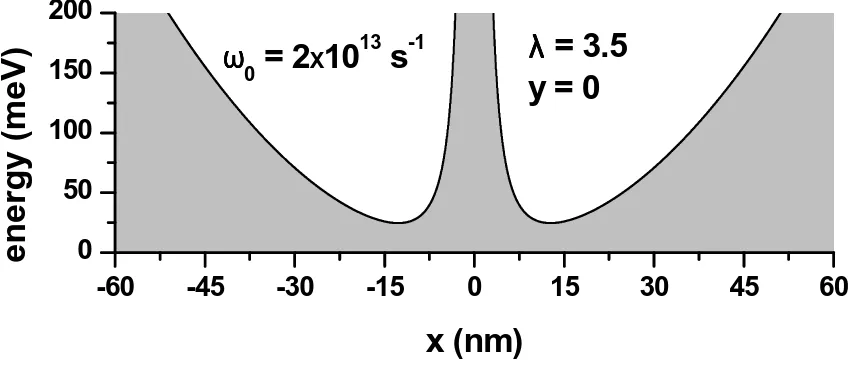
[image:19.612.116.540.69.252.2]y = 0
Figure 3.1: A cross-view showing the potential energy profile along the directionφ= 0.
Knowing that ∇ ×A = B = Bk, we can find thatˆ A = (Ar = 0, Aϕ = Br2 , Az = 0), which is the vector potential of the static magnetic field. We are assuming here the presence of a confining potential,V(r), which combines a parabolic and inverse squared potential functions;
V(r) =1 2m∗ω
2 0r2+
~2
2m∗ λ
r2, (3.2)
where ω0 represents the confinement frequency and the dimensionless parameter λ characterizes
the strength of the the external field, with λ <0 describing an attractive potential and λ≥0 a repulsive one. In the present work, we takeλ≥0 which enables us to calculate solutions for the lower energy bound since the attractive potential has no lower energy bound.
Now, in order to find the eigenfunctions of our system, we introduce the Schr¨odinger equation has the form
ˆ
Hψ=Eψ. (3.3)
If we replace equation (3.1) in this last equation, we have
[ 1
2m∗ [
p+q cA
]2 +V(r)
]
ψ=Eψ
1 2m∗
[ p2+q
2
c2A 2+q
c(p.A+A.p) ]
ψ+V(r)ψ=Eψ. (3.4)
Sincep=−(i~)∇and if we use the Coulomb gauge (∇.A= 0), we can use the fact that∇.(Aψ) =
A.(∇ψ) + (∇.A)ψ=A.(∇ψ) to write
1 2m∗
[ p2+q
2
c2A 2+ 2q
cA.p ]
ψ+V(r)ψ=Eψ. (3.5)
If now, we note thatA.p=Aϕpϕ=−iB~
2
∂
∂ϕ and replace the expression forAand writepin polar coordinates the Schr¨odinger equation adopts the form
[ − ~
2
2m∗ (∂2
∂r2+
1 r ∂ ∂r + 1 r2 ∂2 ∂φ2 ) +q 2 c2 B2
8m∗r
2
−iB2~∂φ∂ +V(r) ]
ψ=Eψ, (3.6)
ˆ Lz= ~
i ∂
∂φ, (3.7)
we obtain [ − ~ 2 2m∗ ( ∂2
∂r2 +
1 r ∂ ∂r + 1 r2 ∂2 ∂φ2 ) +m∗ω
2
c 8 r
2+ωc
2 Lzˆ +V(r) ]
ψ=Eψ, (3.8)
whereωc =mqB∗c is known as the cyclotron frequency. ReplacingV(r) we have
[ − ~
2
2m∗ ( ∂2
∂r2 +
1 r ∂ ∂r + 1 r2 ∂2 ∂φ2 ) +m∗ω
2
c 8 r
2+ωc
2 Lzˆ + 1 2m
∗ω2
0r2+
~2
2m∗ λ r2
]
ψ=Eψ. (3.9)
If we manipulate the terms 1 2m∗ω
2 0r2+
m∗ω2
c
8 r 2= 1
2m∗
( ω2 0+ ω2 c 4 )
r2and define Ω =√ω2 0+
ω2
c
4 as
the total confinement frequency in the magnetic field we arrive to
[ − ~
2
2m∗ ( ∂2
∂r2 +
1 r ∂ ∂r + 1 r2 ∂2 ∂φ2 ) +1
2m∗Ω
2r2+ ~2
2m∗ λ r2 +
ωc 2 Lzˆ
]
ψ=Eψ, (3.10)
where E is the energy eigenvalue. To find the solution of (3.10) that corresponds to a two-dimensional eigenstateψ, it is customary to propose
ψ(r, φ) =R(r)e imϕ √
2π, (3.11)
wheremis an integer usually named as magnetic quantum number, so
[ − ~ 2 2m∗ ( ∂2
∂r2 +
1 r ∂ ∂r − m2 r2 ) +1 2m
∗Ω2r2+ ~2
2m∗ λ r2 +
ωc 2 m~
] R(r)e
imϕ √
2π =ER(r) eimϕ √
2π. (3.12)
Canceling equal terms in both sides of the equation,
[ − ~
2
2m∗ (∂2
∂r2 +
1 r ∂ ∂r − m2 r2 ) +1
2m∗Ω
2r2+ ~2
2m∗ λ r2 +
ωc 2 m~
]
R(r) =ER(r). (3.13)
Manipulating the form of this equation, we can write
[( ∂2 ∂r2 +
1 r ∂ ∂r − m2 r2 ) −m∗
2Ω2
~2 r 2
−rλ2 −
ωcmm∗
~
]
R(r) =−2m~2∗ER(r). (3.14)
We can perform an additional substitution as
R(r) = χ(r)√r , (3.15)
and use it to calculate ∂
∂rR(r) and ∂2
∂r2R(r) as
∂
∂rR(r) = ∂χ(r)
∂r r
−1/2−1
2χ(r)r
−3/2, (3.16)
and
∂2
∂r2R(r) =
∂2χ(r)
∂r2 r− 1/2
−∂χ(r)∂r r−3/2+3 4χ(r)r
−5/2, (3.17)
The combination of (3.14-3.17) allows to obtain an equation forχ(r) in the form
d2χ
dr2 +
[2m∗ E
~2 −
m∗Ω2
~2 r 2
−m
2+λ−1/4
r2
]
with
E=E−m~2ωc. (3.19)
Now, if we perform a typical change, which consist of settingl(l+ 1) =m2+λ−1/4, we have
d2χ
dr2 +
[2m∗ E
~2 −
m∗Ω2
~2 r 2
−l(lr+ 1)2 ]
χ= 0, (3.20)
where the only solution of the quadratic equation forlwith physical meaning is:
l=−1 2 +
√
λ+m2. (3.21)
Introducing a new variable asρ=r2 we can write
d dr = 2ρ
1/2 d
dρ, (3.22)
and
d2
dr2 = 2
d dρ+ 4ρ
d2
dρ2, (3.23)
then, it is possible to rewrite the differential equation (3.20) as follows;
d2χ
dρ2 +
1 2ρ
dχ dρ−
[m∗2Ω2
4~2 +
l(l+ 1) 4ρ2 −
m∗E 2~2ρ
]
χ= 0. (3.24)
Definingη=√ ~
m∗Ω,κ= 2~EΩ,sm=
l+1 2 =
1 4+
√ λ+m2
2 and setting ρ=η
2zwe have
d dρ =
1 η2
d
dz, (3.25)
and
d2
dρ2 =
1 η4
d2
dz2. (3.26)
With the last changes, equation (3.24) can be written as
d2χ
dz2 +
1 2z dχ dz − [ 1 4 +
sm(sm−1/2)
z2 −
κ z ]
χ= 0. (3.27)
Taking into account the asymptotic behavior at the origin and at the infinity for the wave function, we can propose the following ansatz for the well-defined solutions at those two limits:
χ(z) =zsm
e−z/2F(z), (3.28)
where we can obtain
dχ(z) dz =smz
sm−1
e−z/2F(z)
−12zsm
e−z/2F(z) +zsm
e−z/2dF(z)
dz , (3.29)
and
d2χ(z)
dz2 = z
sm
e−z/2d2F(z)
dz2 + 2smz
sm−1
e−z/2dF(z)
dz −z sm
e−z/2dF(z)
dz
−smzsm−1
e−z/2F(z) +1
4z sm
e−z/2F(z) +sm(sm
−1)zsm−2
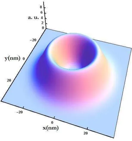
Figure 3.2: The probability density corresponding to the ground state wave function obtained from eqns. (13), (15), and (16). The values ofω0andλare the same used in the figure 1.
Introducing (3.28-3.30) in (3.27) we find the equation
zd
2F
dz2 + ((2sm+ 1/2)−z)
dF
dz −(sm+ 1/4−κ)F = 0, (3.31)
which can be rewritten as
zd
2F
dz2 + (b−z)
dF
dz −aF= 0, (3.32)
known as Kummer’s differential equation, whose solution is the confluent hypergeometric function [36]. Here b = 2sm+ 1/2 and a=sm+ 1/4−κ. The solutions of this equation that guarantee that χ(z) remains finite require the parametera to become a negative integer,−n. In this case, the confluent hypergeometric function reduces to a polynomial ofn-th degree. Here, we are going to use the representation
F(−n, b;x) =Γ(1 +n)Γ(b) Γ(b+n) L
b−1
n (x), (3.33)
where Γ(c) is the Euler gamma function, andLb−1
n (x) are the so-called associated Laguerre poly-nomials. With the aid of (3.11) and (3.33) we can write
ψ(r, φ)mn= Nmn√r r2sm
e−r2/2η2
L2sm−1/2
n (r2/η2)eimϕ, (3.34)
where the normalization constant is determined by means of
∫
dV ψψ∗=|Nmn|2∫ 2π 0
dφ ∫ ∞
0
dr r4sm
e−r2/η2[
L2sm−1/2
n (r2/η2) ]2
= 1, (3.35)
but
∫ 2π
0
dφ= 2π, (3.36)
therefore
2π|Nmn|2 ∫ ∞
0
dr r4sm
e−r2/η2[
L2sm−1/2
n (r2/η2) ]2
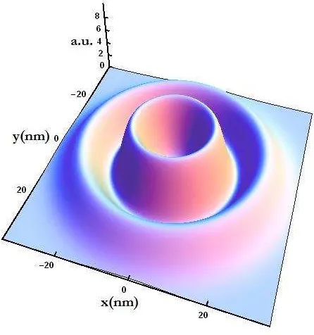
Figure 3.3: The same as in figure 2, but for the case of the wave function that corresponds to the first excited electron state.
In order to find the normalization constant, lets sety=r2/η2, so dy= 2rdr/η2. Then
2πη4sm+1
|Nmn|2 2
∫ ∞
0
dy y2sm−1/2
e−y[L2sm−1/2
n (y)
]2
= 1. (3.38)
Simplifying the last equation and using the orthonormality condition
∫ ∞
0
xαe−xLα
n(x)Lαm(x)dx=
Γ(n+α+ 1)
n! δnm, (3.39)
allow us to write
πη4sm+1
|Nmn|2Γ(n+ 2smn!−1/2 + 1) = 1. (3.40) TakingNnmas a real constant, we can arrive to
Nmn= √
n!
πΓ(2sm+n+ 1/2)η4sm+1. (3.41)
By combiningn=−a= E
2~Ω−sm− 1
4 andE=E−
m~ωc
2 , we can obtain
n= E 2~Ω−
m~ωc
4~Ω −sm−
1 4 =
E 2~Ω−
mωc
4Ω −sm− 1
4, (3.42)
hence
E
2~Ω =n+sm+
1 4+
mωc
Ω . (3.43)
So, the energy spectrum of the confined states as
E= (2n+ 2sm+1 2)~Ω +
m~ωc
2 (3.44)
Replacing the expression forsmand Ω, we can obtain (after settingE=Emn)
Emn= (2n+ 1 +√λ+m2)~
√ ω2
0+
ω2
c 4 +
m~ωc
As it can be seen from the figure 1, if λ ̸= 0, there will be a spatial region in the disc shaped quantum dot in which the repulsive potential barrier centered at the origin is significantly high, and strong enough to keep the electrons far from reaching values of the radial component close to r = 0. This means that the behavior of the carrier system will largely resemble that of the electrons confined in a quantum ring. This is confirmed by observing the figures 2 and 3, where we are depicting the probability density corresponding to the ground and first excited electron states in the system under study. There, the shape of |ψ|2 indicates that the radial region around the
origin is forbidden for the carriers given the repulsive effect of the inverse square barrier. Then, the use of the present model, with a suitable combination of bothω0 andλcould be useful for the
simulation of actual quantum rings, provided the advantages of having analytical expressions for both the wave functions and eigenvalues of the problem.
3.2 Non-Linear Optics
Among the many applications that these states may have, we choose in this work to apply them in the calculation of linear and nonlinear optical coefficients in DSQD (or –as commented above– parabolic 2D QR) provided this kind of systems are attracting much interest in optoelectronics. Given that some intersubband energy intervals, together with their corresponding dipole matrix elements, will be used to calculate the absorption coefficients, we will choose here the energy levels and the wave functions participating in the transition as
E1=E00 E2=E11, ψ1=ψ00 ψ2=ψ11, (3.46)
we then have
E1= (1 +
√ λ)~ √ ω2 0+ ω2 c
4 , (3.47)
and
E2= (3 +
√ λ+ 1)~
√ ω2 0+ ω2 c 4 + ~ωc
2 . (3.48)
The analogous expressions for the wave functions are
ψ1= N√00
rr
2s0e−r2/2η2L2s0−1/2
0 (r2/η2), (3.49)
and
ψ2=
N11
√ rr
2s1e−r2/2η2L2s1−1/2
1 (r2/η2)eiϕ. (3.50)
The energy differenceE21 betweenE2andE1, is expressed as:
E21=E2−E1= (2 +
√
λ+ 1−√λ)~
√ ω2 0+ ω2 c 4 + ~ωc
2 . (3.51)
If we manipulate the expression√λ+ 1−√λas
√
λ+ 1−√λ = ( √
λ+ 1−√λ)(√λ+ 1 +√λ) √
λ+ 1 +√λ λ+ 1−λ
√
λ+ 1 +√λ =
1 √
λ+ 1 +√λ, (3.52)
we are able to obtain
E21=
(
2 +√ 1 λ+ 1 +√λ
) ~ √ ω2 0+ ω2 c 4 + ~ωc
Finally, the electric dipole transition matrix elements are written as
M12=|q⟨ψ1|rcosφ|ψ2⟩|. (3.54)
By the moment, lets focus our attention in calculating the term⟨ψ2|rcosφ|ψ1⟩, which is given by
⟨ψ1|rcosφ|ψ2⟩=N00N11
∫ 2π
0
dφeiϕcosφ ∫ ∞
0
dr r2(s0+s1+1/2)e−r2/η2L2s0−1/2
0 (r2/η2)L 2s1−1/2
1 (r2/η2),
(3.55) but
∫ 2π
0
dφ eiϕcosφ=∫
2π
0
dφ eiϕ(eiϕ+e−iϕ)
2 =
1 2
∫ 2π
0
dφ(e2iϕ+ 1) = 2π
2 =π, (3.56)
then
⟨ψ1|rcosφ|ψ2⟩=N00N11π
∫ ∞
0
dr r2(s0+s1+1/2)e−r2/η2L2s0−1/2
0 (r2/η2)L 2s1−1/2
1 (r2/η2). (3.57)
Taking into account thatL2s0−1/2
0 (r2/η2) = 1, we have
⟨ψ1|rcosφ|ψ2⟩=N00N11π
∫ ∞
0
dr r2(s0+s1+1/2)e−r2/η2L2s1−1/2
1 (r2/η2). (3.58)
Definings0+s1+ 1/2 =α1−1 and 2s1−1/2 =α2, we can write
⟨ψ1|rcosφ|ψ2⟩=N00N11π
∫ ∞
0
dr r2(α1−1)e−r2/η2Lα2
1 (r2/η2), (3.59)
and settingr2/η2=xwhich implies thatdr=dxη
2x−1/2. Therefore
⟨ψ1|rcosφ|ψ2⟩= N00N11πη 2α1−1
2
∫ ∞
0
dx xα1−3/2e−xLα2
1 (x). (3.60)
Using the relation
∫ ∞
0
dx xβ1−1e−xLβ2
n (x) =
(β2−β1+n)!
n!(β2−β1)!
Γ(β1), (3.61)
equation (3.60) becomes
⟨ψ1|rcosφ|ψ2⟩=N00N11πη 2α1−1
2
(α2−α1+ 3/2)!
(α2−α1+ 1/2)!Γ(α1−1/2). (3.62)
Replacing the expressions fors1 ands2 and combining (3.54) and (3.62) we arrive to
M12=|q⟨ψ2|rcosφ|ψ1⟩|=
qπ
2 N00N11η
2(s0+s1+1)(s1−s0−1/2)!
(s1−s0−3/2)!
Γ(s0+s1+ 1). (3.63)
With the idea of calculating the other matrix elements that appear in the optical coefficients of interest, i.e. M11andM22, we must take into account that the factor∫
2π
0 dφcosφ= 0 appears in
those terms. Therefore, we immediately conclude that
M22=M11= 0, (3.64)
which can be thought as a consequence of the electric dipole selection rules.
If use now the results of the last chapter and also and, if we take into account (3.64), the expressions for the linear and third-order nonlinear optical absorption coefficients are, respectively,
α(1)(ω) =ω √µ
ϵR
|M12|2σv~γ12
(E21−~ω)2+ (~γ12)2
and
α(3)(ω) =− √ µ
ϵR
( 4Iω
2ϵ0nrc
)
|M12|4σv~γ12
[(E21−~ω)2+ (~γ12)2]2
, (3.66)
where –as we mentioned in the last chapter– σv is the electron density of the DSQD, µ is the permeability of the system,ϵR=ϵ0n2r(nris the refractive index) is the real part of the permittivity,
~ω is the incident photon energy, andI = 2ϵ0nrcE˜2 is the incident optical intensity. Therefore,
the total optical absorption coefficients can be written as
α(ω) =α(1)(ω) +α(3)(ω). (3.67)
In a similar manner it is possible to obtain the linear and third-order nonlinear relative refractive index change whose expressions are, respectively,
∆n(1)(ω)
nr =
σv|M12|2
2n2
rϵ0
E21−~ω
(E21−~ω)2+ (~γ12)2
(3.68)
and
∆n(3)(ω)
nr =−
σvµcI|M12|4
n3
rϵ0
E21−~ω
[(E21−~ω)2+ (~γ12)2]2
, (3.69)
where (3.64) was again taken into account. Finally the total relative refractive index change can be calculated as
∆n(ω) nr =
∆n(1)(ω) nr +
∆n(3)(ω)
nr . (3.70)
3.3 Results and discussion
In this section we present our calculations for the optical absorption and refractive index change in the type of 2D-quantum dot under study. The prototypical system considered consists of a GaAs-based DSQD, and the values of the confining potential input parameters are those reported in the caption linked to figure 4. Moreover, the different constants appearing in the expressions above are: σv = 5×10²²m−3, Γ
0 = 1/(0.14ps),c= 3 × 10⁸m/s(the speed of light in vacuum),
ϵ0= 8.85×10⁻¹²F/m,µ= 1.256,×10−6T m/A,nr= 3.2,q= 1.6×10⁻¹⁹C, andm∗= 0.067m0,
wherem0 is the free electron mass.
In the figure 3.4(a) one can observe the behavior of the linear, third-order nonlinear and total optical absorption coefficients, calculated as functions of the photon energy. Several distinct values of the applied static magnetic field have been taken into account, as it may be seen from the different curves presented. From the results depicted it is possible to conclude that, as it should be expected, the the main contributions come from the linear term since the third-order coefficient just induces a comparatively small contribution. There is a resonant peak located in~ω = E21
which suffers a blue shift as there is a raising in the magnetic field intensity. By considering the expression (16) for the energy levels, one sees that E21 directly depends on ωc; that is, with the
field amplitude,B. Therefore, when there is an increase of the field intensity, the effect is to move the resonant energy towards higher energy values.
On the other hand, in the figure 3.4(b) we notice the variation of the maximum peak intensity of the coefficients as a function of the magnetic field. Here, the combination of two main reasons can explain the variation in the peak intensities: On one side, we have the variation associated to changes in the value of the electric dipole matrix element|M12|. This quantity tends to decrease
10 20 30 40 50 60 70 -30
10 50 90 130
0 10 20 30
-30 -25 -20 -15 -10 80 100 120 140
(a) 10 T 15 T 5 T
αααα
(
c
m
-1 )
photon energy (meV)
αααα(1)
αααα(3)
αααα
B = 0
(b)
αααα
(
c
m
-1 )
magnetic field (T)
αααα(1)
αααα(3)
[image:27.612.220.433.69.468.2]αααα
Figure 3.4: Linear (black line), third-order nonlinear (red line) and total (blue line) opti-cal absorption coefficients as a function of the photon energy (a) and magnetic field (b) with ω0= 1.2×10¹³s−1,λ= 0.5, andI= 1.5×10¹⁰W/m2 for figure (a). In figure (b) we use the same
parameters as well as~ω=E21.
we realize that the peak intensities vary as a result of the magnetic field provided that the coefficients are proportional to the frequency of resonance,E21, and this quantity grows linearly for sufficiently
high magnetic field strengths, as can be deduced from the equation (18). Such energy difference does not have an upper limit value, therefore we may characterize it as the most influent factor in the behavior of the peak intensities. This is true because it affects mainly the dependence of the linear optical absorption coefficient, which dominates in the overall result. The third-order coefficient contributes more significantly in the region of small field intensities, in which the increase of the energy differenceE21 is the main factor in the variation. Then, for larger field strength, the
decreasing tendency of the dipole matrix elements becomes the leading effect in the monotony of the nonlinear optical absorption coefficient. It is possible to see that the first and total coefficients tend to have the same behavior but it is more visible as we reach sufficiently high magnetic fields due to the fact that at such large values ofB, the contribution ofα(3) is practically negligible.
10 20 30 40 50 60 70 -0.010
-0.005 0.000 0.005 0.010
0 10 20 30
-0.002 0.000 0.002 0.004 0.006 0.008
(a)
15 T 10 T 5 T
∆∆∆∆
n
/
n
photon energy (meV)
∆∆∆∆n(1)
∆∆∆∆n(3)
∆∆∆∆n B = 0
∆∆∆∆n(1)
∆∆∆∆n(3)
∆∆∆∆n
(b)
∆∆∆∆
n
/
n
[image:28.612.221.434.65.457.2]magnetic field (T)
Figure 3.5: Linear (black line), third-order nonlinear (red line) and total (blue line) relative refractive index change as a function of the photon energy (a) and magnetic field (b) with ω0 = 1.2×10¹³s−1, λ = 0.5, and I = 1.5×10¹⁰W/m2 for figure (a). In figure (b) we use
the same parameters as well as~ω=E21−~Γ0.
as well as total relative change, all depicted as functions of the incident photon energy. Again, a set of different values of the magnetic field strength are used as input parameters. According to the discussion made above, augmenting the field intensity leads to a blue shift in the positions of the peaks since, as can be seen from equations (30) and (31), these quantities are directly related with the differenceE21−~ω. Also, one readily observes that, contrary to the case of the optical
absorption coefficients, the growth in the magnitude ofBhas the consequence of a reduction in the ∆n/npeak amplitudes. Looking once again at the same two equations we realize that the variation responsible for such a dependence is that of|M12|vs~ω=E21. Now, there is no factor proportional
to ω that can influence on the value of the coefficients. Therefore, the monotonous evolution of the dipole matrix elements towards a smaller limiting value for high enough field strengths dictates the observed behavior. One may readily notice that by observing the figure 3.5(b). There, the magnitude of the linear, nonlinear and total resonant peak amplitudes are shown as decreasing functions ofB; thus confirming the above made discussion.
5 10 15 20 25 30 35 -40
0 40 80 120
0.0 0.2 0.4 0.6 0.8 1.0 -60
-30 0 30 60 90 120 150
λλλλ
λλλλ
(a)
λλλλ = 0.4
λλλλ = 0.5
λλλλ = 0.6
αααα
(
c
m
-1 )
photon energy (meV)
αααα(1)
αααα(3)
αααα
(b)
αααα
(
c
m
-1 )
λλλλ
αααα(1)
αααα(3)
[image:29.612.219.435.70.473.2]αααα
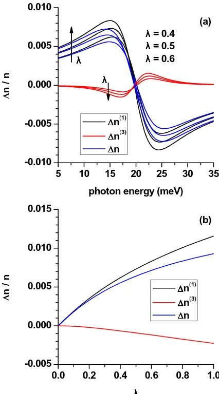
Figure 3.6: Linear (black line), third-order nonlinear (red line) and total (blue line) optical absorp-tion coefficients as a funcabsorp-tion of the photon energy (a) and the dimensionless parameterλ(b) with ω0 = 1.2×10¹³s−1, B = 0, and I = 1.5×10¹⁰W/m2 for figure (a). The direction of the arrows
determines in which direction is raising λfor the optical absorption coefficients. In figure (b) we use the same parameters as well as~ω=E21.
constant, and vary the dimensionless parameterλ. As a consequence of this, there is observed a a non perceptible red shift of the resonant peak but the sizes of the peaks do present significant variations. At a first glance, it is possible to see that when λ increases its value, not only the first-order peak increases its size but also the third-order peak does it. This behavior allows us to conclude that when the inverse square potential parameter acquires sufficiently large values, the confinement potential is strong enough as to prevent us from neglecting the contribution of the third order coefficient –even if the first order contribution is significantly stronger. The variation of the peak intensities can be explained on the basis of the arguments presented in the comments about Fig. 3.4. But this time we must clarify that the matrix element|M12|tends to grow as we increase
λ, whereas the energy differenceE21decreases withλgiven that it has an inverse dependence on it.
However, it should be stressed that, in this situation, the role of dominant quantity is represented by |M12|; which explains why also in this case, the peaks tend to increase their intensities with
5 10 15 20 25 30 35 -0.010
-0.005 0.000 0.005 0.010
0.0 0.2 0.4 0.6 0.8 1.0
-0.005 0.000 0.005 0.010 0.015
λλλλ λλλλ
(a)
λλλλ = 0.4
λλλλ = 0.5
λλλλ = 0.6
∆∆∆∆
n
/
n
photon energy (meV)
∆∆∆∆n(1)
∆∆∆∆n(3)
∆∆∆∆n
(b)
∆∆∆∆n(1)
∆∆∆∆n(3)
∆∆∆∆n
∆∆∆∆
n
/
n
[image:30.612.220.433.66.450.2]λλλλ
Figure 3.7: Linear (black line), third-order nonlinear (red line) and total (blue line) relative re-fractive index change as a function of the photon energy (a) and the dimensionless parameter λ (b) withω0 = 1.2×10¹³s−1,B = 0, andI = 1.5×10¹⁰W/m2 for figure (a). The direction of the
arrows determines in which direction is raisingλ for the the corresponding coefficients. In figure (b) we use the same parameters as well as~ω=E21−~Γ0.
contribution to the total coefficient. In fact, it shows a linear increment after certain value of λ that is nearly the same value at which the linear and total optical absorption coefficients begin to show different behaviors.
A similar procedure of calculation, in this case for the relative change in the refractive index of the system, leads to the results shown in the figure 3.7. It can be seen that, in this case, the first and third order contributions have similar behaviors in regard of the variation of the peak amplitudes, as a consequence of the increment in the value of the inverse square potential parameter λ. As in Fig. 3.6(a), there is a non perceptible red shift in the curves. The first-order peak amplitude augments in the positive direction whilst the third-order peak amplitude diminishes (grows along the negative direction) [Fig. 3.7(a)]. The curves shown in the figure 3.7(b) confirm such features. One notices that the influence of augmenting the intensity of the inverse square potential reflects differently for the first- and third-order contributions of this quantity. The explanation for the variations exhibited by ∆(1)/nand ∆(3)/n follows the same arguments presented in the discussion of the results in figure 6. However, it is possible to observe that the third-order coefficient ∆(3)/n
10 20 30 40 0
20 40 60 80
0 20 40 60 80 100 0
20 40 60 80 100
Ι = χ Ι = χ Ι = χ
Ι = χ X 1010 W/m2 (a)
6.0 4.5 3.0
αααα
(
c
m
-1 )
photon energy (meV)
χχχχ = 1.5
ω ω ω
ω0000 = ϑ = ϑ = ϑ = ϑ X 1013 s-1 (b) 4.8 3.6 2.4
ϑϑϑϑ = 1.2
αααα
(
c
m
-1 )
[image:31.612.221.434.68.481.2]photon energy (meV)
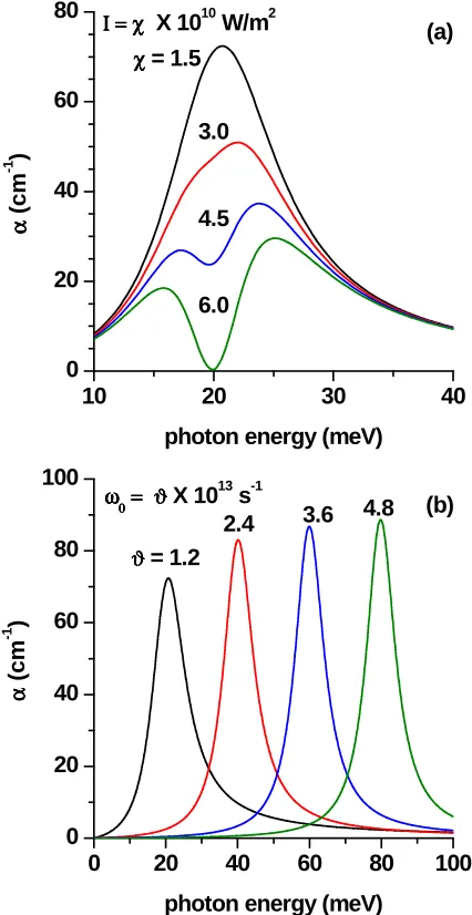
Figure 3.8: Total optical absorption coefficient as a function of the photon energy. In both figures we use λ = 0.5, and B = 0. In figure (a) we use ω0 = 1.2×10¹³s−1 and vary the intensity I
through a parameterχ asI=χ×1010W/m2. In figure (b) we use I= 1.5×10¹⁰W/m2and vary
ω0 through a parameterϑasω0=ϑ×1013s−1.
as with the corresponding dependence of the third-order optical absorption coefficient. We may see from equations (18), (30), and (31) that ∆n/nis, in first-order, proportional toλ1/2, whereas
it becomes proportional toλ3/2 in the case of the third-order contribution. Given that the values
considered for the inverse square parameter are less than unity, this dependence explains the lowest rate of changing for the latter.
10 20 30 40 -0.008
-0.004 0.000 0.004 0.008
0 20 40 60 80 100
-0.008 -0.004 0.000 0.004 0.008
Ι = χ Ι = χ Ι = χ
Ι = χ X 1010 W/m2 (a)
6.0 4.5 3.0
χχχχ = 1.5
∆∆∆∆
n
/
n
photon energy (meV)
ω ω ω
ω0000 = = = = ϑϑϑϑ X 1013 s-1 (b)
4.8 3.6
ϑϑϑϑ = 1.2
2.4
∆∆∆∆
n
/
n
[image:32.612.220.433.72.452.2]photon energy (meV)
Figure 3.9: Total relative refractive index change as a function of the photon energy. In both figures we useλ= 0.5, andB= 0. In figure (a) we useω0= 1.2×10¹³s−1and vary the intensityI
through a parameterχ asI=χ×1010W/m2. In figure (b) we use I= 1.5×10¹⁰W/m2and vary
ω0 through a parameterϑasω0=ϑ×1013s−1.
incident light intensity. Thus, its values remain unchanged if we modify the value of such input quantity. however, the third-order coefficient has a linear dependence withI which implies that as we increase the intensity, the magnitude of this coefficient grows, with –given the negative sign of this contribution– the consequent reduction of the total absorption peak height. It comes a moment when the value of the incident light intensity is so high that the total response at the frequency value of resonance turns to zero, as we may observe in the lowest curve of figure 3.8(a). Moreover, as the effect of increasing the intensity is more apparent, two different peaks begin to appear, in each case with different heights. This is a consequence of the dominant role played by the third-order coefficient, under such conditions.
In the figure 3.8(b) we are representing the curves for the total optical absorption coefficient, obtained by only varying the confinement frequency of the system, ω0. It is possible to observe
a blue shift in the resonant peak. Such an effect can be understood by looking at the expression forE21 given in the equation (18). The increase in ω0 directly reflects in a raising of the energy
difference. The second observed effect is the increasing of the peak intensity associated with the growth of the ω0 value. This is mainly due to the fact that both the first- and third-order
that, as we already discussed, increases with the confinement potential energy. In this particular case, the electric dipole matrix element |M12| tends to decrease as a function of augmenting ω0,
leading us to conclude that, under the conditions present in the evaluation, the term proportional to the energy difference is the leading one, with dominance over the effect introduced by the term proportional to the electric dipole moment.
Under the same conditions taken into account to derive the results shown in the figure 3.8, we have obtained the corresponding variations of the relative change in the refractive index. They are presented in the figure 3.9. The influence of the variation in the incident light intensity appears in fig. 3.9(a), which depicts the total ∆n/n as a function of the photon energy. In this case, one observes that augmenting the value of I results, in a progressive reduction in the resonant peak amplitudes. Once again, this can be explained by considering the increasing contribution coming from the third-order correction, which is the only one term depending on the light intensity –in a linear form. This term is always opposite in sign to the first-order one; thus its weight is progressively carrying importance into the total relative change. However, as we can see, the influence of this nonlinear term is –at least for the values of I considered here– not sufficient to invert the overall monotony of the quantity of interest, which is imposed by the dominance of the –intensity independent– linear contribution and ∆n/n keeps the same functional shape obtained for a fixed value of the incident intensity, and shown in figures 3.5 and 3.7.
The figure 3.9(b) presents the calculated relative change of the refractive index as a function of the incident photon energy with the variation of the degree of confinement posed by the parabolic potential term amplitude. We see now that, together with the blue shift of the resonant peaks, due to the direct dependence of the zero-correction frequencyω=E21/~on the value of the confinement
frequency,ω0. Nonetheless, the peak amplitudes are reduced by the influence of a higher degree of
Conclusions
In this work we have shown that the problem of finding the one-electron conduction states in a two-dimensional disc-shaped quantum dot with parabolic confinement, under the combined influence of an external magnetic field and an inverse square repulsive potential, has an exact analytical solution in the effective mass approximation. According to the symmetry of the obtained eigenstates, this particular potential energy configuration can be used to model the situation of parabolically confined quantum rings in 2D via a suitable choice of the involved parameters.
We have taken advantage of the states and energies so calculated to evaluate the intersubband linear and nonlinear contributions to the optical absorption coefficient as well as to the relative change in the index of refraction in the system under study. The results obtained reveal that the influence of the distinct input elements leads to different behaviors of these two quantities. In general, the augmenting values of both the magnetic field intensity and the parabolic confining amplitude have repercussions in the form of a blueshift of their resonant peaks. On the other hand, the increment in the amplitude of the inverse square potential reflects in an increment of the peak intensities for both coefficients. Finally, augmenting the intensity of the incident light, while remaining the other input elements with fixed values, makes the contribution coming from the third-order nonlinear terms to become more relevant, which causes an overall decrease in the resonant peak amplitudes in both the optical absorption and the refractive index relative variations.
The geometry of the system we have considered and the presence of the magnetic field perpendicular to the plane of the heterostructure makes this an excellent candidate for the calculation of other properties in the system such as: i) the presence of persistent currents and their dependence on geometry, which in this case by appropriate choice of the parameters of potential may be modulated from quantum disks to narrow quantum rings through wide quantum rings, ii) the absorption and photoluminescence spectra associated to magnetoexcitons, iii) the calculation of donor and acceptor properties for impurities confined in the heterostructure, and finally, iv) the effects of in-plane applied electric fields and hydrostatic pressure which can be used to amplify by several orders of magnitude the amplitude of the resonant peaks associated with the different nonlinear optical properties. Some of these works are currently under development and will be published elsewhere.
Bibliography
[1] V. K. Arora and H. N. Spector. Electrical and optical properties of parabolic semiconducting quantum wells. Surface Science176, 669 (1986).
[2] L. Brey, N. F. Johnson, and B. I. Halperin. Optical and magneto-optical absorption in parabolic quantum wells. Phys. Rev. B40, 10647 (1989).
[3] L. Brey, J. Dempsey, N. F. Johnson, and B. I. Halperin. Infrared optical absorption in imperfect parabolic quantum wells. Phys. Rev. B42, 1240 (1990).
[4] K. X. Guo and S. W. Gu. Nonlinear optical rectification in parabolic quantum wells with an applied electric field. Phys. Rev. B47, 16322 (1993).
[5] S. Mukhopadhyay and A. Chatterjee. Rayleigh-Schrdinger perturbation theory for electron-phonon interaction effects in polar semiconductor quantum dots with parabolic confinement. Physics Letters A204, 411 (1995).
[6] X. Hong Qi, X. Jun Jong, and J. J. Li. Effect of a spatially dependent effective mass on the hydrogenic impurity binding energy in a finite parabolic quantum well. Phys. Rev. B58, 10578 (1998).
[7] L. Zhang and H. J. Xie. Electric field effect on the second-order nonlinear optical properties of parabolic and semiparabolic quantum wells. Phys. Rev. B 68, 235315 (2003).
[8] L. Zhang. Electric field effect on the linear and nonlinear intersubband refractive index changes in asymmetrical semiparabolic and symmetrical parabolic quantum wells. Superlatt. Microstruct. 37, 261 (2003).
[9] G. Wang and K. Guo. Interband optical absorptions in a parabolic quantum dot. Physica E 28, 14 (2005).
[10] C. Zhang and K. X. Guo. Polaron effects on the third-order nonlinear optical susceptibility in asymmetrical semi-parabolic quantum wells. Physica B 383, 183 (2006).
[11] S. Elagoz, R. Amca, S. Kutlu, and I. Sokmen. Shallow impurity binding energy in lateral parabolic confinement under an external magnetic field. Superlattices and Microstructures 44, 802 (2008).
[12] S. Wu. Exciton binding energy and excitonic absorption spectra in a parabolic quantum wire under transverse electric field. Physica B406, 4634 (2011).
[13] P. M. Petroff, A. Lorker, and A. Imamoglu, Phys. Today54, 46 (2001).
[14] D. Bimberg, M. Grundman, and N. N. Ledentsov,Quantum Dot Heterostructures(John Wiley Sons, Chichester, 1999).
[15] O. Benson, C. Santori, M. Pelton, and Y. Yamamoto. Regulated and Entangled Photons from a Single Quantum Dot. Phys. Rev. Lett.84, 2513 (2000).