Analysis of chemical bonding and aromaticity from electronic delocalization descriptors

Texto completo

(1)ANALYSIS OF CHEMICAL BONDING AND AROMATICITY FROM ELECTRONIC DELOCALIZATION DESCRIPTORS. Ferran FEIXAS GERONÈS. Dipòsit legal: GI-1023-2011 http://hdl.handle.net/10803/37471. ADVERTIMENT. La consulta d’aquesta tesi queda condicionada a l’acceptació de les següents condicions d'ús: La difusió d’aquesta tesi per mitjà del servei TDX ha estat autoritzada pels titulars dels drets de propietat intel·lectual únicament per a usos privats emmarcats en activitats d’investigació i docència. No s’autoritza la seva reproducció amb finalitats de lucre ni la seva difusió i posada a disposició des d’un lloc aliè al servei TDX. No s’autoritza la presentació del seu contingut en una finestra o marc aliè a TDX (framing). Aquesta reserva de drets afecta tant al resum de presentació de la tesi com als seus continguts. En la utilització o cita de parts de la tesi és obligat indicar el nom de la persona autora. ADVERTENCIA. La consulta de esta tesis queda condicionada a la aceptación de las siguientes condiciones de uso: La difusión de esta tesis por medio del servicio TDR ha sido autorizada por los titulares de los derechos de propiedad intelectual únicamente para usos privados enmarcados en actividades de investigación y docencia. No se autoriza su reproducción con finalidades de lucro ni su difusión y puesta a disposición desde un sitio ajeno al servicio TDR. No se autoriza la presentación de su contenido en una ventana o marco ajeno a TDR (framing). Esta reserva de derechos afecta tanto al resumen de presentación de la tesis como a sus contenidos. En la utilización o cita de partes de la tesis es obligado indicar el nombre de la persona autora. WARNING. On having consulted this thesis you’re accepting the following use conditions: Spreading this thesis by the TDX service has been authorized by the titular of the intellectual property rights only for private uses placed in investigation and teaching activities. Reproduction with lucrative aims is not authorized neither its spreading and availability from a site foreign to the TDX service. Introducing its content in a window or frame foreign to the TDX service is not authorized (framing). This rights affect to the presentation summary of the thesis as well as to its contents. In the using or citation of parts of the thesis it’s obliged to indicate the name of the author..

(2) PhD thesis:. Analysis of Chemical Bonding and Aromaticity from Electronic Delocalization Descriptors. Ferran Feixas Geronès 2010 Doctorat Interuniversitari en Quı́mica Teòrica i Computacional PhD supervisors: Prof. Miquel Solà i Puig Dr. Jordi Poater i Teixidor Dr. Eduard Matito i Gras Memòria presentada per a optar al tı́tol de Doctor per la Universitat de Girona.

(3) El professor Miquel Solà i Puig, catedràtic d’Universitat a l’àrea de Quı́mica Fı́sica de la Universitat de Girona, el doctor Jordi Poater i Teixidor, investigador Ramón y Cajal a l’Institut de Quı́mica Computacional de la Universitat de Girona, i el doctor Eduard Matito i Gras, investigador postdoctoral Marie-Curie de l’Institut de Fı́sica de la University of Sczczecin.. CERTIFIQUEM: Que aquest treball titulat ”Analysis of Chemical Bonding and Aromaticity from Electronic Delocalization Descriptors”, que presenta en Ferran Feixas Geronès per a l’obtenció del tı́tol de Doctor, ha estat realitzat sota la nostra direcció i que compleix els requeriments per a poder optar a Menció Europea.. Signatura. Prof. Miquel Solà Puig. Dr. Jordi Poater i Teixidor. Girona, 1 de desembre de 2010. Dr. Eduard Matito i Gras.

(4) ”I quan penses dur a terme el teu somni? -va demanar el mestre al deixeble. Quan tingui la oportunitat -va respondre. El Mestre li contestà -L’oportunitat mai no arriba. L’oportunitat és aquı́.” Anthony de Mello. A tots vosaltres. v.

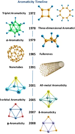
(5) Preface Since the advent of quantum mechanics, theoretical and computational chemistry have played a pivotal role in chemistry. From the very beginning, theoretical chemists have been primarily focused on the development of new methodologies that may provide an explanation for most of the chemical phenomena. However, progress in the applicability of theoretical and computational chemistry depends on the advances in computational power. This fact limited the interaction between experimental and theoretical chemists for a long time. Notwithstanding, at the end of the first decade of the 21st century, we have arrived at a position where theory and experiment play a complementary role in exploring chemical questions. Theoretical chemistry is now commonly used to address complex problems in chemistry, biochemistry, or materials science, from the study of small molecules in the gas phase to the simulation of protein folding in complex environments. 1 Interactions between electrons determine the structure and properties of matter from molecules to solids. Therefore, the understanding of the electronic structure of molecules will enable us to extract relevant chemical information. Since the work of Lewis, 2 the concept of electron pair has been placed at the epicenter of the discussion about the properties of chemical bonding. Hence, the pair density, that accounts for the correlated motion of a couple of electrons, has been very important in the interpretation of electronic structure. The pair density and its related quantities, such as the concept of Fermi Hole, are discussed in detail in Chapter 1. Interestingly, these quantities have been widely used to elucidate the nature of chemical bonding in a plethora of systems. In chemistry, global molecular properties are as important as the properties of a given atom or region of the molecular space. The partition of molecular space into different regions helps us to unravel how the electrons are localized in a specific region or which is the number of electrons shared among two or more regions of the space. In Chapter 2 we will see how we can more clearly understand the nature of chemical bonding from the concept of electron delocalization. From the discovery of benzene in 1825 3 to the present day, the concept of aromaticity has experienced several revolutions that have fueled the interest of both theoretical and experimental chemists. The discovery of new aromatic compounds is not about to slow down. Undoubtedly, the major breakthrough of the last decade in the field of aromaticity took place in 2001, when the first all-metal cluster, M Al4− (M = Li, Na, or Cu), was characterized. 4 This finding gave rise to one of the most vii.

(6) striking features of all-metal aromatic clusters, the so-called multifold aromaticity, that is, the presence of σ-, π-, δ-, or even φ-aromaticity. As the number of new aromatic molecules grows, the quest for the quantification of aromaticity has become one of the challenges of theoretical chemists. Thus, the concept of aromaticity is one of the cornerstones of past and current chemistry. However, at the same time, it is also considered a chemical unicorn 5 due to the fact that aromaticity is not a directly measurable property, and it cannot be defined unambiguously. In Chapter 3, the main advances in the field and the most widely used descriptors of aromaticity will be reviewed. On the other hand, Chapters 5, 6, and 7 are devoted to the applications of the above presented theory and correspond to the works of the present thesis, that contains twelve accepted publications. First, we focus our attention on the analysis of chemical bonding by means of the Electron Localization Function (ELF) 6 and the Domain-Averaged Fermi Hole analysis (DAFH). 7,8 The four projects collected in Chapter 5 are a consequence of the research stays at the Université Pierre et Marie-Curie with Prof. Bernard Silvi, and at the Czech Academy of Science with Prof. Robert Ponec. In the first section, the ELF is approximated in terms of natural orbitals in order to bridge the gap between the (expensive) correlated expression and the (sometimes inaccurate) monodeterminantal definition. The next sections are dedicated to DAFH analysis. First, this analysis is generalized to open-shell systems; second, the open-shell definition is used to analyze the bonding patterns of some triplet dications; and, third, the peculiarities of the ultrashort Cr-Cr bond are analyzed from the point of view of DAFH. In recent years, many methods to quantify aromaticity based on different physicochemical properties have been proposed. In Chapter 6 we assess the performance of these indicators by analyzing their advantages and drawbacks. Throughout this chapter, we propose a series of tests based on well-known aromaticity trends that can be applied to evaluate the aromaticity of current and future indicators of aromaticity in both organic and inorganic species. Since the aromaticity is tightly connected with the concept of electron delocalization, in Chapter 7 we investigate the nature of electron delocalization in both aromatic and antiaromatic systems in the light of Hückel’s (4n + 2) rule. Finally, from the conclusions gathered in Chapter 6, we analyze the phenomenon of multiple aromaticity in all-metal clusters that present σ, π, and/or δ aromaticity.. viii.

(7) Resum de la tesi Des del sorgiment de la mecànica quàntica, la quı́mica teòrica i computacional ha jugat un paper fonamental en el món de la quı́mica. Des de bon principi, els quı́mics teòrics s’han centrat en el desenvolupament de noves metodologies que poden proporcionar una explicació per a la majoria de fenómens quı́mics. No obstant, els avenços en l’aplicació de la quı́mica computacional han estat molt lligats als avenços en el camp de la computació. Aquest fet ha limitat la interacció entre els quı́mics experimentals i teòrics durant gran part del segle XX. Tot i això, al final de la primera dècada del segle XXI, hem arribat a una posició on la teoria i l’experiment juguen un paper complementari en l’exploració de tot tipus de problemes quı́mics. La quı́mica teòrica s’ha convertit en una eina d’ús comú per fer front a problemes complexos que abarquen camps com la quı́mica o la bioquı́mica, des de l’estudi de molècules petites en fase gasosa a la simulació del plegament de proteı̈nes. 1 Les interaccions entre electrons determinen l’estructura i propietats de la matèria. Per tant, la comprensió de l’estructura electrònica de les molècules ens permetrà extreure informació quı́mica rellevant. Des del treball de Lewis, 2 el concepte de parell d’electrons es troba a l’epicentre de la discussió sobre les propietats de l’enllaç quı́mic. Per tant, la densitat de parells, que representa el moviment correlacionat d’un parell d’electrons, ha jugat un paper clau en la interpretació de l’estructura electrònica. Les propietats de la densitat de parells i les seves quantitats associades, com ara el forat de Fermi, es discutiran en detall al Capı́tol 1. Aquestes quantitats s’han utilitzat àmpliament per desentrallar la naturalesa de l’enllaç quı́mic en una gran quantitat de sistemes. En quı́mica, tan importants com les propietats globals de la molècula ho són les propietats d’un átom o una regió de l’espai molecular. La partició de l’espai en diferents regions pot ajudar-nos a esbrinar com es localitzen el electrons dins una regió especı́fica o quin és el nombre d’electrons compartits entre dues o més regions de l’espai. En el Capı́tol 2 veurem com podem analitzar la naturalesa de l’enllaç quı́mic a partir del concepte de deslocalització electrònica. Des del descobriment de la molècula de benzè l’any 1825 3 fins a l’actualitat, el concepte d’aromaticitat ha experimentat diverses revolucions que han provocat l’interès dels quı́mics teòrics i experimentals. El descobriment de nous compostos aromàtics no para d’augementar exponencialment. Sens dubte, el gran avanç de l’última dècada en el camp de l’aromaticitat es va dur a terme l’any 2001, quan el primer compost totalment metàl·lic amb propietats aromàtiques va ser caracteritzat, M Al4− (M = Li, Na, o Cu). 4 Aquesta troballa va donar lloc a una de les caracterı́stiques més ix.

(8) sorprenents del anells aromàtics formats per només metalls: l’anomenada aromaticitat múltiple, és a dir, la presència d’aromaticitat de tipus σ, π, δ, o fins i tot φ. Com que el nombre de noves molècules aromàtiques no para de créiexer, la recerca per la quantificació de l’aromaticitat s’ha convertit en un dels reptes dels quı́mics teòrics. Aixı́ doncs, el concepte d’aromaticitat és una de les pedres angulars de la quı́mica actual, però al mateix temps, també és considerat un unicorn quı́mic, 5 degut a que l’aromaticitat no és una propietat directament mesurable, i per tant no es pot definir sense ambigüitat. Al Capı́tol 3 revisarem els principals avenços en el camp de l’aromaticitat i els seus descriptors més utilitzats. D’altra banda, els Capı́tols 5, 6, i 7 estan dedicats a les aplicacions d’aquesta tesi, que conté un total de dotze publicacions acceptades. En primer lloc, centrem la nostra atenció en l’anàlisi de l’enllaç quı́mic per mitjà de la funció de localització electrònica (ELF) 6 i l’anàlisi dels anomenats domain averaged Fermi holes (DAFH). 7,8 Els quatre projectes recollits en el Capı́tol 5 són conseqüència de les estades de recerca realitzades a la Université Pierre et Marie Curie amb el Prof. Bernard Silvi, i a l’Acadèmia Txeca de les Ciències amb el Prof. Robert Ponec. A la primera secció, proposem una aproximació de la ELF en termes d’orbitals naturals per tal de reduir la distància entre l’expressió a nivell correlacionat que porta associat un elevast cost computacional i la definició (moltes vegades inexacta) basada en funcions d’ona monodeterminantals. Les següents seccions estan dedicades a l’anàlisi dels DAFH. En primer lloc, aquest anàlisi s’ha generalitzat a sistemes de capa oberta, en segon lloc, la definició dels DAFH a capa oberta s’utilitza per analitzar els patrons d’enllaç d’alguns dications en estat triplet, i, en tercer lloc, les peculiaritats dels enllaços extremadament curts de Cr-Cr s’analitzen des del punt vista dels DAFH. En els últims anys, s’han proposat molts mètodes per quantificar l’aromaticitat basats en diferents propietats fisicoquı́miques. En el Capı́tol 6 s’avalua el comportament d’aquests indicadors analitzant els seus avantatges i inconvenients. Al llarg d’aquest capı́tol, es proposen una sèrie de tests basats en tendències d’aromaticitat conegudes que es poden aplicar per avaluar el comportament dels indicadors actuals en espècies tan orgàniques com inorgàniques. Com que l’aromaticitat està estretament vinculada amb el concepte de deslocalització electrònica, en el Capı́tol 7 s’investiga la naturalesa de la deslocalització d’electrons en sistemes aromàtics i antiaromàtics que segueixen la regla 4n + 2 que proposà Hückel. Finalment, a partir de les conclusions reunides al Capı́tol 6, analitzarem el fenomen de l’aromaticitat múltiple en sistemes metàl·lics que presenten aromaticitat de tipus σ, π, i δ. x.

(9) Agraı̈ments ”Caminante, no hay camino se hace camino al andar” Antonio Machado Sempre he pensat que el doctorat és com fer el Camı́ de Santiago, cada matı́ agafes les bici, vas fent etapes, coneixes gent, nous llocs, i tot i saber quin és l’objectiu final saps que el que és veritablement important és viure el dia a dia, l’avui, l’aquı́ i l’ara. Ara que comença l’últim tram de l’última etapa, la il·lusió per arribar al final queda enterbolida per una barreja de sentiments, per una banda l’alegria per tots els moments viscuts, per tot el que he après, i per l’altra la tristesa de saber que s’acaba una etapa genial. Si que és cert que al llarg del camı́ hi ha algun Cebreiro o Creu de Ferro amb pendent del 20% que t’obliga a baixar pinyons i a apretar fort les dents, però un cop has coronat el cim valores tot l’esforç i rius recordant tots els entrebancs de la pujada. Però si alguna cosa he après al llarg d’aquests anys de doctorat és que molt més important que els resultats obtinguts són les persones que t’acompanyen i que et vas trobant al llarg de la caminada. Les persones que t’ajuden, amb els qui rius, que t’animen, en definitiva, els qui et fan fàcil el camı́, o dit d’una altra manera, les persones que fan que cada moment, que cada dia, sigui especial i diferent. Que sapigueu que de tots vosaltres n’estic constantment aprenent. En aquestes lı́nies no podré agrair-vos la meitat del que voldria ni la meitat del que us mereixeu. Abans de res, moltes gràcies a tots! En primer lloc, vull donar les gràcies als tres responsables que això hagi tirat endavant, els directors de la tesi, Miquel, Jordi i Edu. No veig la tesi com un premi individual sinó com un el premi a un treball d’equip. Us vull agrair el vostre recolzament en tot moment, el vostre entusiasme, els infinits consells, per dirigir-me sempre cap a la direcció correcte i perquè he pogut aprendre constantment de tots vosaltres. Particularment, a en Miquel voldria donar-li les gràcies perquè sense ell possiblement no hauria escrit aquesta tesi ni estaria fent actualment el doctorat, ja que va ser a partir de tenir-lo de professor, que en gran part s’em va despertar un interés real per seguir amb la quı́mica teòrica. A en Jordi, coodirector de la tesi, vull agrair-li especialment haver-me donat la oportunitat d’entrar dins el món de la biomedicina. Si he pogut demanar els projectes de les beques per anar de postdoc ha estat gràcies a en Jordi, ja sigui tan per ajudar-me a definir el projecte com per totes les correccions xi.

(10) i comentaris posteriors. A l’Edu, coodirector de la tesi, però per sobre de tot un amic, agrair-li en primer lloc totes les hores, que espero que no siguin perdudes, que ha dedicat a explicar- me tot tipus de conceptes al llarg d’aquests cinc anys. També pels infinits consells, xerrades de tots tipus, sopars a base de feta cheese al millor bar d’Atenes, congressos, converses futboleres... Gràcies a tots tres per la vostra paciència, per aguantar els meus despistes i per ajudar-me en tot moment. A tots tres moltes gràcies, he estat aprenent constantment de vosaltres i ho continuaré fent. No em voldria oblidar de l’Annapaola i en Lluı́s, ja que m’han ofert la possibilitat d’endisar-me en el fascinant món de la fotoquı́mica, dels mecanismes de reacció impossibles i de les conicals intersections entre estats ultraexcitats, i també per la oportunitat d’anar a Jena d’estada, gràcies per totes les hores dedicades! També a en Marcel per tota la seva ajuda amb el tema LUCTA, que per un neòfit de l’ADF i del món MM com jo va ser difı́cil. A la resta del sector IQCcià, als séniors, Josep Maria, Sı́lvia, Emili, Miquel Duran, Ramon, Sergei, Alexander, especial menció a la Carme, per contrarrestar tot lo despistats que podem ser en el tema papeleo i per fer-nos riure sempre que baixem al bar. Després d’haver voltat molt per Europa t’adones de que veritablement no hi ha enlloc com a casa i això és gràcies a vosaltres, l’IQC és com una famı́lia i sempre pensaré que és el millor grup on he pogut estar. Voldria agrair a en Bernard, en Robert i la Leticia perquè m’han tractat com a casa en les estades que he fet. A Bernard quiero agradecerle la estancia de cuatro meses a Paris, por todo lo que pude aprender acerca de ELF y ToPMoD, por los increibles cous-cous que comı́amos cerca del laboratorio, y porque coincidimos en que la Bretanya francesa es de los mejores sitios del mundo. I want to thank Robert for his hospitality throughout the two months that I spent in Prague, for all that I learned about DAFH, for his guided tours (every tuesday after lunch) to the most incredible places of one of the best cities in Europe, for the delicious lunch with his family at his place, for the three apples that I found every morning on the table, and finally, for give me the opportunity to carry out a research stay in the research center with the best cantine of the world, long live dumplings! Finalmente, agradecer a Leticia y a todo su grupo por la estancia en Jena, llegar el dı́a 10 de enero a -25 grados no fue fácil, pero en seguida me sentı́ como en casa, también quiero agradacer particularmente a Vero y a Suso por toda su ayuda y paciencia en el tema de les dinámicas. Especial menció als erasmus de Paris i a la colla de l’Spanisch Stammtisch de Jena per tots els bons moments, sopars, etc Merci beaucoup! Vielen danke! xii.

(11) Be, arribat a aquest punt toca centrar-me amb tota la colla de freaks (o amics) amb qui hem compartit infintat de bons moments i aventures de tot tipus. Tot va començar al 177 (l’origen de tot nou Iqcià), amb el treball experimental. Tot estava tan col·apsat que en Dani (l’immortal del 177) ocupava mitja taula i jo l’altre meitat. Després, un grup d’irreductibles iqcians vam emprendre un llarg viatge cap a la conquesta de noves terres, a l’altra banda de la muntanya, on hem viscut grans moments. No em vull deixar ningú, tots vosaltres també sou part de la tesi (sense vosaltres potser l’hauria acabat abans ;) (esto es roja no??) però no m’ho hauria passat tan bé): a la Sı́lvia (la meva germana gran a l’IQC), en Pata (el meu germà fotoquı́quimic), Dani (com es pot ser tan freak), Juanma (gestor de l’Univers i explotador de becaris de 1r any (algú ho havia de dir)), Lluı́s (Ramb... no he dit! Independència o no?), Cristina (freak multidimensional), Dachs (gadgetocàmera sempre a punt), Diaz (màxima potència sobre la bici), Mireia (la mama del despatx), Eloy (Chygramos-Córdoba), Pedro (Peeeetraaaa!), Oscar (compadre y mı́stico que s’está gelant a Suècia), Samat (more wine? wine not), Yevhen (els seus - què significa...?originen discusions interminables al despatx), David (de les Xungues), Quansong (Quantum Li, com va això?), Albert (la Roca, el mestre dels blocks), Torrentxu (sempre a l’avantguarda de la música), Quim (algun xiste més?) i també a tota la nova generació d’iqcians Carles, Majid, Sergi, Laia, Mickael, Luz i Marc, estar a l’IQC trastoca, oju! Només de recordar tots els bons moments se’m posa la pell de gallina: els kebabs ultrapicants i les partides interminables de pocha de manchesterliverpool, el cuba bar i la secta herbalife de Colonia, les migdiades als parcs i les llargues estones al centre comercial (mallrats!) de Goteborg, l’atac de les gavines assassines de Helsinki, els dominis propis d’Amsterdam, el feta cheese d’Atenes, l’espicha d’Oviedo. Però també els freaks de la bici (que casi no ho expliquen), els freaks de can Miá (ja toca no?), els freaks del 177 (Se ha matao Paco!), els freaks del jocs de taula (com el junglespeed cap), els freaks del japó (Arigatou!), els freaks del futbol (Inda forever!), els freaks de l’apm (ho haveu vist?), hi ha algú normal? Ens ho hem passat i ens ho seguirem passant molt bé! Afegir només que per fi he trobat gent més despistat i impuntual que jo! Si alguna cosa he après és que un no arriba mai tard, sinó que arriba quan s’ho proposa. I com no, no vull oblidar-me de tota la tribu experimental, que tot i que els matxaquem a les jodete son molt bones persones (Mira si es buena persona), pels sopars al basc, els estiu a carpes, etc. Venga pues, arreando que es tarde! Especial menció a la Summerschool de Dinamarca amb la Sı́lvia i en Pata, la veritat xiii.

(12) és que va ser genial, Saatana Perkele!, encuentros en la tercera fase amb en Hussein (quin crack!!!), socialitzant fins a altes hores, en Pisuke (sanhilali), la locomotora Vargas, les hores de problemes amb en Philip Callaghan (how is it going?), les partides al rotten, l’esmorzar, el dinar, els pastissos de berenar, els sopar, la peixera, la sauna, en Hellboy, el caa̧dor de cocodrils (impagable l’escena del projector), en pepe olsen, el tigre de helgaker, en collina, els partits de futbol de 3 hores, el freak que feia problemes fins a les 12 de la nit (quin matat!),... i com no el paper fonamental que va tenir en el viatge el regalı́s (nunca mais). Que consti en acte! No em puc oblidar de la Penya de l’Espardenya! Annes D, Santi, Alba, Naiara, Mònica F, Mònica B, Maira, Marta, Carla, Xevi, Ferram, Pilar, Olga, Quim. Sense vosaltres la carrera no hagués estat el mateix, festes, sopar de gala, viatge a Tunissia, a la biblio fins a les mil de la nit, sopars al suca-mulla, el brie amb pebrots, la peli Vaig Fort, carpes de Girona, els partits de basket de l’es Tio Conco Team. Però sobretot perquè seguim organitzant tot tipus d’events per anar-nos trobant, amics invisibles, sopars de barrakes, .... KUAK!!! Kasikeno Productions presenta... a la colla de Banyoles, Albert, Anna L., Anna P., Chak, David, Edu, Enric, Ester, Fina, Joan, Jordi, Maria L., Maria M., Maria V., Mariona, Miki, Sı́lvia, que us puc dir que no us hagi dit en 18 hores de cotxe seguides per anar a Berlin? Suecia, Frankfurt, Cannes, Madrid, Londres, Berlin, Euskadi, Bretanya, Aquitània, Noruega... Gràcies per totes les hores que hem passat i seguirem passant junts, festes de tot tipus, converses paranoiques a l’Ateneu, tot tipus de concerts, fins i tot un concert insonor!, Marie-Claires, la Trini Sánchez Mata (Trini la que mata), carnavals, ens ho partim?, i com no els grans èxits de la Kasikeno Street Band: fred del nord ja som aquı́, corren rumors rhapsody, que bé que vius, .... no acabaria mai! Perdoneu-me per arribar sempre tard, però quan marxi de postdoc segur que trobeu a faltar els sms ”faig 20 minuts tard”. Last but no least, els més importants, ja que sense ells res seria possible i mai els hi podré agrair prou tot el que han fet per mi. La meva famı́lia, la mare, el pare, en Guillem (des de Porto amb la cesi, la nair i la isis), i als que per mi també són germans, en Milla (i per extensió la Pharbin i en Subó) i la Tabita, a tots vull donar-vos les gràcies per tots els valors que m’heu transmès, per tot el que m’heu permès veure i viure i per ser sempre allà on calia. Moltes vegades no t’adones del valor que tenen les coses fins al cap d’un temps. Les rutes per pràcticament tot Europa amb el volskwagen jetta i tenda, les classes amb els ganduls, els dinars a la xiv.

(13) casa, les converses sobre el Barça amb en Milla, mirar Amelie i Diarios de Motocicleta repetidament amb en Guillem, el viatge que vau fer a Bangladesh per buscar els pares de’n Milla, els consells però sobretot per deixar-me completa llibertat. No m’agradaria oblidar-me dels avis ni de la resta de la famı́lia. Als avis de Banyoles pel seu suport constant, per preocupar-se per mi, per preguntar-me sempre què es el que estic investigant i escoltar-me, ara podré venir més sovint a dinar :). L’ávia de Palafrugell per ser una avia diferent, es la persona que més optimisme i dinamisme m’ha transmès, no havia vist mai ningú amb tantes inquietuds i estic molt orgullós que sigui la meva àvia. Us estimo molt a tots!!. xv.

(14) Full List of Publications The thesis is based on the following publications: Chapter 5 1. Feixas, F.; Matito, E.; Duran, M.; Solà, M.; Silvi, B.; The Electron Localization Function at the Correlated Level: A Natural Orbital Formulation. J. Chem. Theory Comput. 6, 2736-2742, 2010 2. Ponec, R.; Feixas, F.; Domain Averaged Fermi Hole Analysis for Open-shell systems. J. Phys. Chem. A 113, 5773-5779, 2009 3. Feixas, F.; Ponec, R.; Fiser, J.; Schröder, D.; Roithová, J.; Price, S.D.; Bonding analysis of the [C2 O4 ]2+ intermediate formed in the reaction of CO22+ with neutral CO2 . J. Phys. Chem. A 113, 6681-6688, 2010 4. Ponec, R.; Feixas, F.; Peculiarities of Multiple Cr-Cr Bonding. Insights from the analysis of Domain- Averaged Fermi Holes. J. Phys. Chem. A 113, 8394-8400, 2009 Chapter 6 5. Matito, E.; Feixas, F.; Solà, M.; Electron Delocalization and Aromaticity Measures within the Hückel Molecular Orbital Method. J. Mol. Struct. (THEOCHEM) 811, 3-11, 2007 6. Feixas, F.; Matito, E.; Poater, J.; Solà, M.; Aromaticity of Distorted Benzene Rings. Exploring the Validity of Different Indicators of Aromaticity. J. Phys. Chem. A 111, 4513-4521, 2007 7. Feixas, F.; Jiménez-Halla, J.O.C..; Matito, E.; Poater, J.; Solà, M.; Is the aromaticity of the benzene ring in the (η 6 − C6 H6 )Cr(CO)3 complex larger than that of the isolated benzene molecule?. Pol J. Chem. 81, 783- 797, 2007 8. Feixas, F.; Matito, E.; Poater, J.; Solà, M.; On the Performance of Some Aromaticity Indices: A Critical Assessment Using a Test Set. J. Comput. Chem. 29, 1543-1554, 2008 9. Feixas, F.; Jiménez-Halla, J.O.C.; Matito, E.; Poater, J.; Solà M.; A Test to Evaluate the Performance of Aromaticity Descriptors in All-Metal and Semimetal Clusters. An Appraisal of Electronic and Magnetic Indicators of Aromaticity. J. Chem. Theory Comput. 6, 1118-1130, 2010 xvii.

(15) Chapter 7 10. Feixas, F.; Matito, E.; Solà, M.; Poater, J.; Analysis of HückelÕs [4n+2] Rule Through Electronic delocalization measures. J. Phys. Chem. A 112 13231-13238, 2008 special issue: Sason Shaik Festschrift. 11. Feixas, F.; Matito, E.; Solà, M.; Poater, J.; Patterns of π-electron delocalization in aromatic and antiaromatic organic compounds in the light of the HückelÕs [4n+2] Rule. Phys. Chem. Chem. Phys. 12, 7126-7137, 2010 12. Feixas, F.; Matito, E.; Duran, M.; Poater, J.; Solà, M.; Aromaticity and electronic delocalization in all- metal clusters with single, double, and triple aromatic character. Theor. Chem. Acc. Accepted for publication, 2010, in the Special Issue devoted to Theoretical Chemistry in Spain. Publications not included in this thesis: 13. Leyva, V.; Corral, I.; Schmierer, T.; Heinz, B.; Feixas, F.; Migani, A.; Blancafort, Ll.; Gilch, P.; González, L.; Electronic States of o-Nitrobenzaldehide: A Combined Experimental and Theoretical Study. J.Phys. Chem. A 112, 5046, 2008 14. Feixas, F.; Solà, M.; Swart, M.; Chemical bonding and aromaticity in metalloporphyrins. Can. J. Chem. 87, 1063-1073, 2009 in the Special Issue dedicated to Professor T. Ziegler 15. Solà, M.; Feixas, F.; Jiménez-Halla, J.O.C.; Matito, E.; Poater, J.; A Critical Assessment of the Performance of Magnetic and Electronic Indices of Aromaticity. Symmetry 2, 1156-1179, 2010 16. Feixas, F.; Matito, E.; Swart, M.; Poater, J.; Solà, M.; Electron Delocalization in Organometallic Compounds: From Agostic Bond to Aromaticity AIP Conference Proceedings of the International Conference on Computational Methods in Science and Engineering, ICCMSE 2009, AIP, Accepted for publication, 2010 17. Migani, A.; Leyva, V.; Feixas, F.; Schmierer, T.; Gilch, P.; Corral, I; GonzĞlez, L.; Blancafort, Ll; Excited State Hydrogen Transfer in ortho-nitrobenzaldehid: A correlated diagram translated to a conical intersection triangle and cascade, Submitted for publication, 2010. xviii.

(16) List of Acronyms Abbreviation. Description. 1-RDM 2-PD 2-RDM AIM AOM ASE BB BCP BLA BLE CASSCF CBO CCP CCSD CISD CP DAFH DI DFT ELF ESI FBO FLU HEG HF HF-XCD HOMA HMO LI MBO MCI MO MP2. First-order Reduced Density Matrix Two-Particle Density Second-order Reduced Density Matrix Atom In a Molecule Atomic Overlap Matrix Aromatic Stabilitzation Energy Buijse and Baerends approach Bond Critical Point Bond Lenght Alternation Bond Lenght Elongation Complete Active Space Self Consistent Field Coulson Bond Order Cage Critical Point Coupled Cluster Singles and Doubles Configuration Interaction Singles and Doubles Conditional Probability Domain-Averaged Fermi Hole Delocalization Index Density Functional Theory Electron Localization Function Electron Sharing Index Fuzzy-atom Bond Order Aromatic Fluctuation index Homogenous Electron Gas Hartree-Fock Hartree-Fock Exchange-Correlation Density Harmonic Oscillator Model of Aromaticity Hückel Molecular Orbital Localization Index Mayer-Bond Order Multicenter Index Molecular Orbital Second-oder Moller-Plesset Perturbation Theory xxi.

(17) Abbreviation. Description. NCP NICS NNA PDI QTAIM RCP RDM XCD. Nuclear Critical Point Nucleus-independent chemical shifts Non-Nuclear Attractor Para-Delocalization Index Quantum Theory of Atoms in Molecules Ring Critical Point Reduced Density Matrix Exchange-Correlation Density. xxii.

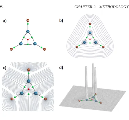
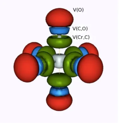
(18) Contents Preface . . . . . . . . . . . Resum de la tesi . . . . . Agraı̈ments . . . . . . . . Full List of Publications List of Acronyms . . . . .. . . . . .. . . . . .. . . . . .. . . . . .. . . . . .. . . . . .. . . . . .. . . . . .. . . . . .. . . . . .. . . . . .. . . . . .. . . . . .. . . . . .. . . . . .. . . . . .. . . . . .. . . . . .. . . . . .. . . . . .. . . . . .. . . . . .. 1 Introduction 1.1 From Quantum Mechanics to Quantum Chemistry . . . . . . . 1.2 A brief overview of Quantum Chemistry . . . . . . . . . . . . 1.3 Physical Interpretation of the Wave Function . . . . . . . . . . 1.4 Density Functions . . . . . . . . . . . . . . . . . . . . . . . . . 1.5 Density Matrices . . . . . . . . . . . . . . . . . . . . . . . . . 1.6 Two-electron Densities and Holes . . . . . . . . . . . . . . . . 1.6.1 Pair Density and Exchange Correlation Density . . . . 1.6.2 Conditional Probability and Pair Correlation Function 1.6.3 Fermi and Coulomb Holes . . . . . . . . . . . . . . . . 2 Methodology 2.1 The Atom in a Molecule . . . . . . . . . . . . . 2.1.1 Quantum Theory of Atoms in Molecules 2.1.2 Fuzzy Atom Schemes . . . . . . . . . . . 2.2 Electron Sharing Indices . . . . . . . . . . . . . 2.2.1 Definition . . . . . . . . . . . . . . . . . 2.2.2 Example: Cr(CO)6 . . . . . . . . . . . . 2.3 Domain-Averaged Fermi Hole Analysis . . . . . 2.3.1 DAFH definition . . . . . . . . . . . . . 2.3.2 Example: Cr(CO)6 . . . . . . . . . . . . 2.4 Electron Localization Function . . . . . . . . . . 2.4.1 Becke’s Definition . . . . . . . . . . . . . xxiii. . . . . . . . . . . .. . . . . . . . . . . .. . . . . . . . . . . .. . . . . . . . . . . .. . . . . . . . . . . .. . . . . . . . . . . .. . . . . . . . . . . .. . . . . . . . . . . .. . . . . . . . . . . . . . . . . . . . . . . . . .. . . . . . . . . . . . . . . . . . . . . . . . . .. . . . . .. . vii . ix . xi . xvii . xxi. . . . . . . . . .. . . . . . . . . .. 1 1 3 5 6 8 10 11 14 15. . . . . . . . . . . .. 21 22 23 29 30 31 38 41 41 44 50 50. . . . . . . . . . . ..

(19) 2.4.2. Example: Cr(CO)6 . . . . . . . . . . . . . . . . . . . . . . . . 53. 3 Aromaticity 59 3.1 Key Advances . . . . . . . . . . . . . . . . . . . . . . . . . . . . . . . 60 3.2 Descriptors of Aromaticity . . . . . . . . . . . . . . . . . . . . . . . . 66 4 Objectives. 75. 5 Applications I: The Nature of the Chemical Bond from Electron Localization Function and Domain-Averaged Fermi Holes 77 5.1 Electron Localization Function at the Correlated Level: A Natural Orbital Formulation . . . . . . . . . . . . . . . . . . . . . . . . . . . 79 5.2 Domain Averaged Fermi Hole Analysis for open-shell systems . . . . . 87 5.3 Bonding Analysis of the [C2 O4 ]2+ Intermediate Formed in the Reaction of CO22+ with Neutral CO2 . . . . . . . . . . . . . . . . . . . . . 95 5.4 Peculiarities of Multiple Cr-Cr bonding. Insights from the Analysis of Domain-Averaged Fermi Holes . . . . . . . . . . . . . . . . . . . . 105 6 Applications II: Critical assessment on the performance of a set of aromaticity indexes 113 6.1 Electron Delocalization and Aromaticity Mesures within the Hückel Molecular Orbital Method . . . . . . . . . . . . . . . . . . . . . . . . 115 6.2 Aromaticity of Distorted Benzene Rings: Exploring the Validity of Different Indicators of Aromaticity . . . . . . . . . . . . . . . . . . . 125 6.3 Is the Aromaticity of the Benzene Ring in the (η 6 − C6 H6 )Cr(CO)3 Complex Larger than that of the Isolated Benzene Molecule? . . . . . 135 6.4 On the Performance of Some Aromaticity Indices: A Critical Assessment Using a Test Set . . . . . . . . . . . . . . . . . . . . . . . . . . 151 6.5 A Test to Evaluate the Performance of Aromaticity Descriptors in All-Metal and Semimetal Clusters. An Appraisal of Electronic and Magnetic Indicators of Aromaticity . . . . . . . . . . . . . . . . . . . 177 7 Applications III: Study of electron delocalization in organic/inorganic compounds 193 7.1 Analysis of Hückel’s [4n + 2] Rule through Electronic Delocalization Measures . . . . . . . . . . . . . . . . . . . . . . . . . . . . . . . . . . 195 7.2 Patterns of π-electron Delocalization in Aromatic and Antiaromatic Organic Compounds in the Light of Hückel’s [4n + 2] . . . . . . . . . 205 xxiv.

(20) 7.3. Aromaticity and electronic delocalization in all-metal clusters with single, double, and triple aromatic character . . . . . . . . . . . . . . 219. 8 Results and Discussion 8.1 Applications I . . . . . . . . . . . . . . . . . . . . . . . . . . . . . . 8.1.1 Electron Localization Function . . . . . . . . . . . . . . . . 8.1.2 Domain-Averaged Fermi Holes . . . . . . . . . . . . . . . . . 8.2 Applications II . . . . . . . . . . . . . . . . . . . . . . . . . . . . . 8.2.1 Electronic Aromaticity indices at HMO level . . . . . . . . . 8.2.2 A Critical Assessment on the Performance of Aromaticity Criteria in Organic Systems . . . . . . . . . . . . . . . . . . . . 8.2.3 A Critical Assessment on the Performance of Aromaticity Criteria in All-Metal Clusters . . . . . . . . . . . . . . . . . . . 8.3 Applications III . . . . . . . . . . . . . . . . . . . . . . . . . . . . . 8.3.1 Electron Delocalization in Organic Systems . . . . . . . . . . 8.3.2 Electron Delocalization in All-Metal Clusters . . . . . . . . . 9 Conclusions. 233 . 233 . 233 . 236 . 247 . 248 . 250 . . . .. 256 259 260 267 271. xxv.

(21) Chapter 1 Introduction: Quantum Mechanics, Density Matrices and Density Functions 1.1. From Quantum Mechanics to Quantum Chemistry. Toward the end of the 19th century, many scientists considered physics as a complete discipline that gave a successful explanation for different natural phenomena and allowed to interpret the results of most of the experiments. The contributions of Galileo and Newton to classical mechanics, or the works of Faraday and Maxwell in the field of electricity and magnetism, signified extremely important advancements in the comprehension of the physical reality, from the large objects of the universe to the quotidian things around us. Quantum Mechanics is at the heart of many areas of physics. This theory plays a critical role in understanding the laws of nature that govern the domain of the small, that is, particles such as electrons, or bigger entities like atoms and molecules. The quantum theory was a rupture with regard to the intuitive way of conceiving the physical world. Do electrons behave like waves or like particles? Or more interestingly, could an electron behave like a particle and a wave at the same time? The works of Max Planck, Erwin Schrödinger, or Werner Heisenberg among many others, firmly established the basis of quantum theory and supposed one of the major breakthroughs of the 20th century. In the realm of quantum mechanics, mathemat1.

(22) 2. CHAPTER 1. INTRODUCTION. ics plays a key role. Thus, the Hilbert space, the abstract algebra, or the theory of probabilities allow to predict the results of many experiments with surprisingly accurate precision. In quantum theory, the scientific predictions of the results are statistical in nature, and are treated in terms of probabilities. Consequently, concepts such as uncertainty, fuzziness, and probability are deeply linked to quantum theory. The determinism that characterized classical mechanics gave way to the indeterminism associated with quantum mechanics. Quantum mechanics has been very successful in accounting for many experimental results in particle physics and in the properties of atoms and molecules. However, the first steps of quantum mechanics were followed by a lengthily discussion about the validity of this theory to describe physical reality. During this period, some authors claimed that quantum mechanics was barely a statistical theory that could not provide a complete description of the physical world and, thus, some variables that would improve the comprehension of the theory must remain occult. For instance, the entanglement phenomena has been at the epicenter of the debate about the incompleteness of the quantum theory. Notwithstanding, the theory was accepted by most of the physical community and played a key role from the very beginning. The discovery of quantum theory found potential applications in other fields of science such as chemistry, giving birth to the area called Quantum Chemistry. The main objectives of this thesis will be addressed from the quantum chemical point of view. At the end of 19th century, great advances in the field of chemistry had been made up to that time. For instance, the initially controversial concept of molecule was finally widely accepted; the impressing work of Mendeleev gave rise to the periodic table of the elements; and Kekulé finally unraveled the structure of benzene. However, the mechanism of how a chemical reaction occurs, or concepts such as the nature of chemical bonding or the aromaticity of a given molecule remained unexplainable. Hence, a heated debate over atoms, molecules, or the early concepts of chemical bonding occupied a central position in the most important conferences before the 20th century. One of the most striking advances was published in 1916 by G. N. Lewis. 2 In that paper, Lewis proposed a model to study the chemical bonding based on the concept of lone and sharing electron pairs. The first steps towards the concepts of electron localization and delocalization were established. Although the Lewis model presents some pitfalls, it has been widely used from the very beginning by most of the chemical community to account for the electronic distribution of a.

(23) 1.2. A BRIEF OVERVIEW OF QUANTUM CHEMISTRY. 3. given molecule. Like physics, chemistry experimented a step forward with the advent of quantum mechanics. Nevertheless, the mathematical complexity associated with quantum chemical calculations distanced experimental chemists from theoretical chemists. This gap was reduced with the fast advances in computational power giving rise to the so-called computational chemistry. Thus, from computational chemistry, it is possible to explore the potential energy surface of complex reactions and describe their reaction mechanism. In addition, the magnetic properties of a large group of molecules could be accurately predicted or the dynamical behavior of biological systems could be analyzed through molecular simulations. Quantum chemistry opened a completely new way to analyze the electronic structure or physical and chemical molecular properties. In the last decades, a large number of new methods has been proposed to improve the conception of chemistry. However, chemists still use some old chemical conceptions such as bonding strength, atomic charges or aromaticity to provide an explanation for different chemical phenomena. Consequently, one of the main aims of several theoretical research groups has been to reconcile these old concepts with quantum mechanics. But how can we use quantum mechanics to evaluate the nature of chemical bonding or the aromaticity of a conflicting system? Will this information help us to predict the stability or reactivity of organic and inorganic molecules, and offer explanations for different chemical phenomena? In the next chapters of this thesis, we will give an overview of the most widely used methods to analyze the chemical bonding and aromaticity.. 1.2. A brief overview of Quantum Chemistry. We will briefly summarize the basic concepts of quantum chemistry that are needed to understand the next sections and chapters. The ultimate goal of quantum chemistry is to find the (approximate) solution of time-independent, non-relativistic Schrödinger equation that gives the description of the statistical behavior of particles: � 1, R � 2 , ..., R � M ) = εi Ψi (�x1 , �x2 , ..., �xN , R � 1, R � 2 , ..., R �M) ĤΨi (�x1 , �x2 , ..., �xN , R. (1.1). where Ĥ is the Hamiltonian operator for a molecular system composed by M nuclei.

(24) 4. CHAPTER 1. INTRODUCTION. and N electrons. The Ĥ contains the kinetic operators, T̂e and T̂N , which describe the kinetic energy of the electrons and nuclei respectively, and three potential operator terms, V̂ee , V̂N e , and V̂N N , that account for both attractive and repulsive potential energies. Each state i is associated with a wave function. Therefore, Ψi is the wave function of the state i of the system which depends on the 3N spatial electronic coordinates (�rN ) and the N electronic spin coordinates (�sN ) that are col� M ). εi are the lectively named as �xN , and the 3M spatial nuclear coordinates (R numerical values of the energy of state i. Consequently, the main aim of quantum chemistry is to solve the Schrödinger equation in order to find the eigenfunctions, i.e. the wave functions Ψi , and the corresponding eigenvalues εi of Ĥ. The wave function, Ψi , contains all the information that can be known about a quantum system. Once the wave function is determined, all properties of interest can be acquired by applying the appropriate operators to the wave function. However, the exact solution of the Schrödinger equation is unaffordable and, thus, there is a need to find different strategies to solve approximately this eigenfunction-eigenvalue problem. The first basic approach, that can be easily applied in most of the cases, is the so-called Born-Oppenheimer approximation. Since the nuclei are much heavier than the electrons and, thus, much slower, it is a good approximation to take the extreme point and consider the electrons as moving in the field of fixed nuclei, as two separated motions. Then, the Born-Oppenheimer approximation evaluates the motions of nuclei and electrons separately, which extremely simplifies the problem. In this way, the Ĥ may be divided into electronic and nuclear terms, Ĥelec and Ĥnuc , and the solutions of the Schrödinger equation with Ĥelec are the electronic wave function Ψelec (�x1 , �x2 , ..., �xN ) and the electronic energy Eelec . Now, the Ψelec explicitly � M . Finally, the total energy depends on the �xN coordinates and parametrically on R Etot is the sum of Eelec and the constant nuclear energy Enuc , which is the nuclear repulsion term of the Ĥ:. � M ) = Eelec Ψelec (�xN ; R �M) Ĥelec Ψelec (�xN ; R. (1.2). Etot = Eelec + Enuc. (1.3). From now on we will only consider the electronic wave function and we will refer to.

(25) 1.3. PHYSICAL INTERPRETATION OF THE WAVE FUNCTION. 5. it as Ψ.. 1.3. Physical Interpretation of the Wave Function. In Quantum Mechanics, concepts such as bond order, atomic charge or aromaticity are not observables, that is, they cannot be directly measured by means of any operator, and therefore, they have no physical direct interpretation. Moreover, the wave function itself is not an observable. Hence, how can we translate the information of quantum theory to shed some light on the nature of these widely used chemical concepts? In 1926, Max Born proposed the physical interpretation of the square of the wave function, |Ψ|2 , in terms of probabilities. This statistical analysis provides the probability to find N particles in a given region: |Ψ(�x1 , �x2 , ..., �xN )|2 d�x1 d�x2 . . . d�xN. (1.4). |Ψ(�x1 , �x2 , ..., �xi , �xj , . . . , x�N )|2 = |Ψ(x�1 , x�2 , ..., �xj , �xi , . . . , �xN )|2. (1.5). Ψ(�x1 , �x2 , ..., �xi , �xj , . . . , x�N ) = −Ψ(x�1 , x�2 , ..., �xj , �xi , . . . , �xN ). (1.6). This equation informs us about the probability of finding simultaneously electrons 1,2,...,N in volume elements d�x1 , d�x2 , ..., d�xN . Due to the fact that electrons are indistinguishable, the exchange of two electron coordinates must not change this probability:. Consequently, there are only two possibilities that when interchanging their coordinates the probability remains unaltered, first, the wave functions are identical or, second, the interchange of two coordinates leads to a sign change. This requirement is fulfilled by two groups of particles. The bosons, which have integer spin and their wave function is symmetric with respect to the interchange of coordinates, and the fermions that have half-integer spin and their switch leads to an antisymmetric wave function. For fermions we have:. Since the electrons are fermions with spin 1/2, we will deal with antisymmetric wave functions. The antisymmetry principle is the quantum-mechanical generalization of Pauli exclusion principle, two electrons with the same spin cannot occupy the same state. Hence, the electrons are constrained by the Pauli exclusion principle. The consequences of this principle have a crucial importance on the localization and.

(26) 6. CHAPTER 1. INTRODUCTION. delocalization of electrons, the main topic of this thesis. As the integral of Eq. 1.4 over the full space equals one, the probability of finding N electrons anywhere in the space must be exactly the unity: �. .... �. |Ψ(x�1 , x�2 , ..., x�N )|2 dx�1 dx�2 . . . dx�N = 1. (1.7). To sum up the information presented up to now, in classical physics we can, in principle, measure, determine and predict, for instance, the position and the velocity of a moving object with full precision. On the other hand, in quantum mechanics the predictions are statistical in nature, and, for instance, we can study the probability of finding a portion of particles like electrons in a given region. This portion of electrons can be associated with the concept of electronic charge and, thus, with the so-called electron density. Consequently, the square of the wave function leads to both the electron density and the pair density, which are one-particle and twoparticle electron distributions, respectively. The information given by the density and the pair density can be translated to acquire the electronic structure of a given molecule and, hence, one can study properties such as the chemical bonding or the aromaticity of a plethora of systems.. 1.4. Density Functions. In this section, the concepts of electron density and pair density are defined. We have a system with N electrons which is described by a wave function, Ψ(�x1 , �x2 , ..., �xN ). As previously mentioned, the product of Ψ(�x1 , �x2 , ..., �xN ) with its complex conjugate Ψ∗ (�x1 , �x2 , ..., �xN ) gives the probability of finding electron 1 between �x1 and �x1 + d�x1 , while electron 2 is between �x2 and �x2 + d�x2 , ..., and electron N is between �xN and �xN + d�xN . It is particularly interesting to study the probability of finding electron one regardless of the position of the remaining N − 1: d�x1. �. Ψ(�x1 , �x2 , . . . , �xN )Ψ∗ (�x1 , �x2 , . . . , �xN )d�x2 . . . d�xN. (1.8). since the electrons are indistinguishable the probability of finding one electron is ρ(�x1 ) = N d�x1. �. Ψ(�x1 , �x2 , . . . , �xN )Ψ∗ (�x1 , �x2 , . . . , �xN )d�x2 . . . d�xN. (1.9). where ρ(�x) is the so-called density function. The integration of Eq. 1.9 with respect.

(27) 1.4. DENSITY FUNCTIONS. 7. to the spin coordinates leads us to the probability density, which is known as the electron density, ρ(�r): ρ(�r1 ) =. �. ρ(�x1 )ds1. = N d�x1. �. Ψ(�x1 , �x2 , . . . , �xN )Ψ∗ (�x1 , �x2 , . . . , �xN )d�s1 d�x2 . . . d�xN (1.10). The electron density is the angular stone of density functional theory (DFT) due to the fact that it contains all the information needed to describe the energy of the ground state of a given molecule. As opposed to the wave function, the electron density is an observable and can be measured experimentally by means of X-ray diffraction. Since Ψ is normalized, and the electrons are indistinguishable, the integration over the whole space is N , that is, the total number of electrons: �. ρ(�r1 )d�r1 = N. (1.11). For the sake of clarity, the electron density can also be represented as ρ(�x1 ) = γ (1) (�x1 ). (1.12). The definition of the pair density is also interesting. The concept of electron pair is the cornerstone of Lewis’ model and will play a crucial role in methodologies devoted to the analysis of chemical bonding. The probability of finding electrons 1 and 2 in the volume elements �x1 and �x2 is given by. d�x1 d�x2. �. Ψ(�x1 , �x2 , . . . , �xN )Ψ∗ (�x1 , �x2 , . . . , �xN )d�x3 . . . d�xN. γ (2) (�x1 , �x2 ) = N (N − 1). �. (1.13). Ψ(�x1 , �x2 , . . . , �xN )Ψ∗ (�x1 , �x2 , . . . , �xN )d�x3 . . . d�xN (1.14). The pair density is a two-particle electron distribution which informs us about the probability density of finding a certain couple of electrons, e.g. 1 and 2, irrespective of the position of the remaining N − 2 electrons. The interpretation is analogous to the one given by the electron density of finding one electron in a particular region. One can also define a spinless pair density:.

(28) 8. CHAPTER 1. INTRODUCTION. γ (2) (�r1 , �r2 ) =. 1.5. �. γ (2) (�x1 , �x2 )ds1 ds2. (1.15). Density Matrices. As previously mentioned, the N -electron wave function obtained by solving the Schrödinger equation for a many-particle system contains all the possible information about the quantum state. This wave function, that it is very difficult to obtain, includes a large amount of information that will not be employed at all. Thus, from this wave function is usually too complicated to provide a simple physical picture of the system. Notwithstanding, it is possible to use alternative mathematical structures called reduced density matrices. These density matrices are simpler than the wave function itself and have a more direct physical meaning. For instance, the two-electron reduced density matrix (2-RDM) comprises all the physically and chemically important information. In principle, the 2-RDM can be used to compute the energy and the atomic and molecular properties without the need of the many-particle wave function. 9 However, there are some conditions, such as the N representability, which has to be fulfilled to ensure that the 2-RDM derives from the N -electron wave function. This field has potential applications in many areas of physics and chemistry, e.g., it could represent a bridge between the density functional theory and the ab initio wave function methods. 10 From the N-electron wave function, Ψ(�x1 , . . . , �xN ), one can define the N -order density matrix (DM) as γ (n) (�x1 � . . . �xN �|�x1 . . . �xN ) = Ψ∗ (�x1 �, . . . , �xN �)Ψ(�x1 , . . . , �xN ). (1.16). where N is the number of electrons in our system. This matrix depends upon 2N variables which is beyond feasible computations with current computers. The number of variables is reduced to construct the m-order reduced density matrices, by integration of N − m of its coordinates: γ. (m). �. �. � n (�x1 � . . . �xm �|�x1 . . . �xm ) = m! m. γ (n) (�x1 � . . . �xm �, �xm+1 . . . �xN |�x1 . . . �xN ) ΔN xm+1 . . . �xN m+1 d�. (1.17).

(29) 1.5. DENSITY MATRICES. 9. where ΔN m+1 is the generalized Dirac delta. ΔN m+1. N �. =. i=m+1. δ(�xi � − �xi ). (1.18). The first-order (1-RDM) reduced density matrices are particularly interesting: γ (1) (�x1 �|�x1 ) = N. �. Ψ∗ (�x1 � . . . �xm �, �xm+1 . . . �xN )Ψ(�x1 , . . . , �xN )ΔN x2 . . . �xN (1.19) 2 d�. and also the second-order reduced density matrices: γ (2) (�x1 ��x2 �|�x1�x2 ) = N (N − 1). �. Ψ∗ (�x1 � . . . �xm �, �xm+1 . . . �xN )Ψ(�x1 , . . . , �xN ). ΔN x3 . . . �xN 3 d�. (1.20). Let us now show how we can use the m-RDM in order to compute the density functions described in the above section. The wave function can be expanded in terms of Slater determinants: Ψ=. �. cK ψK. (1.21). K. where ψK are the Slater determinants constructed from a set of orthonormalized spin orbitals: 1 ψK = √ |χ1 (�x1 ), χ2 (�x2 ), . . . , χN (�xN )| N!. (1.22). In this case, Eq. 1.17 can be further simplified to obtain γ (m) (�x1 � . . . �xm �|�x1 . . . �xm ) =. �. i1 i2 ...im j1 j2 ...jm. ...jm ∗ Γji11ij22...i χi1 (�x1 �), . . . χ∗im (�xm �)χj1 (�x1 ), . . . χjm (�xm ) m. (1.23). ...jm Thus, the m-RDM is calculated as an expansion of our basis set. The Γji11ij22...i m is computed from the coefficients cK given in Eq. 1.21. For our purposes, it is particularly interesting to further simplify Eq. 1.23 by only taking into account the diagonal terms of the m-RDM, i.e., xi = xi �. Then, we get the m-order density.

(30) 10. CHAPTER 1. INTRODUCTION. functions γ (m) (�x1 . . . �xm ) =. �. ...jm ∗ Γji11ij22...i χi1 (�x1 ), . . . χ∗im (�xm )χj1 (�x1 ), . . . χjm (�xm ) (1.24) m. i1 i2 ...im j1 j2 ...jm. Consequently, we can express the one-electron density as γ (1) (�x1 ) =. �. χ∗i (�x1 )Γji χj (�x1 ). (1.25). i,j. And the two-electron density, which is used to study the electron correlation, is represented in the following manner γ (2) (�x1 , �x2 ) =. �. χ∗i (�x1 )χ∗j (�x2 )Γkl x1 )χl (�x2 ) ij χk (�. (1.26). i,j k,l. ...jm It is worth noticing that the algorithm needed to obtain Γji11ij22...i was designed in our m laboratory by Dr. Eduard Matito in order to calculate the Configuration Interaction Simples and Doubles (CISD) first and second order density matrices. This program has been extended in this thesis to generate the m-order density matrices from the Complete Active Space Self Consistent Field (CASSCF) (see Chapter 5.1 for further applications).. In the case of monodeterminantal wave functions, the density matrices must be diagonal regardless of the order of the matrix. In particular, we can express the p-RDM in terms of 1-RDM: γ (m) (�x1 � . . . �xm �|�x1 . . . �xm ) =. 1.6.        . γ (1) (�x1 �|�x1 ) . . . γ (1) (�x1 �|�xp ) .. .. .. . . . (1) (1) γ (�xp �|�x1 ) . . . γ (�xp �|�xp ). Two-electron Densities and Holes.        . (1.27). The pair density contains all the information referring to the correlated motion of two electrons. The correlation between same spin electrons is called exchange while the correlation due to different spin electrons is called Coulomb correlation. The exchange correlation arises from the antisymmetry of the wave function. At the Hartree-Fock level, the exchange correlation is the only one taken into account,.

(31) 1.6. TWO-ELECTRON DENSITIES AND HOLES. 11. while the Coulomb correlation is neglected. The effect of the Coulomb correlation can be accounted for by means of second-order perturbation theory, configuration interaction (CI), or Coupled Cluster (CC) methods among others. The DFT also introduces these correlation effects but in a different manner. The same information regarding the correlation of electrons is found in other quantities derived from the pair density, such as the exchange correlation density and in the conditional probability.. 1.6.1. Pair Density and Exchange Correlation Density. The pair density can be decomposed in terms of an uncorrelated density and another part that accounts for the electron correlation (both exchange and Coulomb correlations): γ (2) (�x1 , �x2 ) = γ (1) (�x1 )γ (1) (�x2 ) + γXC (�x1 , �x2 ). (1.28). where the first term corresponds to a fictitious pair density constructed as a product of two independent electron distributions, and the second is the so-called exchange correlation density (XCD), γXC (�x1 , �x2 ). 11 The XCD represents the difference between the probability density of finding two electrons, one at x1 and the other at x2 , in a correlated and uncorrelated fashion. As γ (1) (�x1 ) integrates to N and γ (2) (�x1 , �x2 ) to N (N − 1), the integration of this quantity over the whole space gives the total number of electrons −N :1 � �. γXC (�x1 , �x2 )d�x1 , d�x2 ) = −N. (1.31). 1. The XCD could also be defined as the difference between the uncorrelated and correlated motions of two electrons: γ (2) (�x1 , �x2 ) = γ (1) (�x1 )γ (1) (�x2 ) − γXC (�x1 , �x2 ). (1.29). and then, the integration of this quantity gives: � �. γXC (�x1 , �x2 )d�x1 , d�x2 ) = N. (1.30). This definition has been used in most of the publications of Chapters 5, 6, and 7 to introduce the domain averaged fermi holes and the electron sharing indices..

(32) 12. CHAPTER 1. INTRODUCTION. In the next chapter, we will see the role played by the XCD to assess the electron localization and delocalization between two given atoms, or regions, of the molecular space. Before entering to the world of molecular partition and electron sharing indices, we will see how Eq. 1.29 can be manipulated for monodeterminantal wave functions. In the literature most of the calculations are closed-shell and with monodeterminantal wave functions, using both HF or DFT within the Kohn and Sham formalism, the pair density of Eq. 1.29 can be further simplified in terms of the 1-RDM using Eq. 1.27:. γ. (2). (�x1 � . . . �x2 ) =.     . γ (1) (�x1 |�x1 ) γ (1) (�x1 |�x2 ) γ (1) (�x2 |�x1 ) γ (1) (�x2 |�x2 ). Les us now split Eq. 1.32 in terms of its spins cases:.     . (1.32). γ (2)αα (�r1 , �r2 ) + γ (2)αβ (�r1 , �r2 ) + γ (2)βα (�r1 , �r2 ) + γ (2)ββ (�r1�r2 ) = (γ (1)α (�r1 ) + γ (1)β (�r1 ))(γ (1)α (�r2 ) + γ (1)β (�r2 )) +(γ (1)α (�r1 |�r2 ) + γ (1)β (�r1 |�r2 ))(γ (1)α (�r2 |�r1 ) + γ (1)β (�r2 |�r1 )) = γ (1)α (�r1 )γ (1)α (�r2 ) + γ (1)α (�r1 )γ (1)β (�r2 ) +γ (1)β (�r1 )γ (1)α (�r2 ) + γ (1)β (�r1 )γ (1)β (�r2 ) +γ (1)α (�r1 |�r2 )γ (1)α (�r2 |�r1 ) + γ (1)β (�r1 |�r2 )γ (1)β (�r2 |�r1 ). (1.33). where, after the integration over one coordinate, the cross-spin out-of-diagonal terms of the 1-RDM, γ (1)α (�r1 |�r2 )γ (1)β (�r2 |�r1 ) = 0 due to the orthonormality of the spin functions. Interestingly, in the case of monodeterminantal wave functions, the cross-spins contributions, which are responsible for the Coulomb correlation, come only from the fictitious product of one-electron densities and, thus, the electrons with antiparallel spin move in a completely uncorrelated fashion. This fact has important consequences in the calculation of both the electron localization function and electron.

(33) 1.6. TWO-ELECTRON DENSITIES AND HOLES. 13. sharing indices as we will see in the next chapters. In a large number of cases, the HF approximation dramatically fails, for instance in some strong covalent interactions. Thus, the inclusion of Coulomb correlation is crucial to describe the electronic structure of the system. As previously mentioned, the calculation of the exact pair density is usually unaffordable. Fortunately, the pair density can be successfully approximated in terms of natural orbitals for correlated wave functions. Some of the most popular approximations have been summarized in the introduction of Chapter 5.1. After bringing together the terms corresponding to the density and pair density, Eq. 1.33 can be simplified as:. γ (2) (�r1 , �r2 ) = γ (1) (�r1 )γ (1) (�r2 ) + γ (1)α (�r1 |�r2 )γ (1)α (�r2 |�r1 ) + γ (1)β (�r1 |�r2 )γ (1)β (�r2 |�r1 ). (1.34). Only in the case of closed-shell monodeterminantal wave functions, the α and β contributions that come from the out-of-diagonal terms of the 1-RDM can be collected together. Thus, the second order density matrix can be obtained from the 1-RDM one: 1 γ (2) (�r1 , �r2 ) = γ (1) (�r1 )γ (1) (�r2 ) + γ (1) (�r1 |�r2 )γ (1) (�r2 |�r1 ) 2. (1.35). Therefore, the spinless version of the XCD within a monodeterminantal wave function is 2 1  (1) r1 |�r2 ) γ (�  γXC (�r1 , �r2 ) =  2. (1.36). This is the expression of the XCD which is used in most of this thesis to calculate the values of the electron sharing indices (see Chapters 6 and 7), where the calculations have been essentially performed at the DFT level within the Kohn-Sham approach with both closed and open-shell monodeterminantal wave functions. From Eq. 1.36, one can generalize the expression of the exact pair density as.

(34) 14. CHAPTER 1. INTRODUCTION. 1 γ (2) (�r1 , �r2 ) = γ (1) (�r1 )γ (1) (�r2 ) + γ (1) (�r1 |�r2 )γ (1) (�r2 |�r1 ) + λ(2) (�r1 , �r2 ) 2. (1.37). where λ(2) (�r2 , �r1 ) is the so-called cumulant matrix. 12 This term was proposed by Kutzelnigg and Mukherjee and accounts for the exact correlation contribution. In Chapter 5.1 this formula has been approximated by means of a natural orbital approach. Thus, at the correlated level, the formula for the XCD can be rewritten as: 1 γXC (�r1 , �r2 ) = γ (1) (�r1 |�r2 )γ (1) (�r2 |�r1 ) + λ(2) (�r1 , �r2 ) 2. (1.38). Obviously, within the framework of HF approximation one has λ(2) (�r1 , �r2 ) = 0.. 1.6.2. Conditional Probability and Pair Correlation Function. As we have seen, the XCD, as the pair density, contains all the information concerning the correlated motion of two electrons. We can go one step further and define the so-called conditional probability (CP). The CP describes the probability of finding electron 2 at position �r2 when electron 1 is fixed at the position �r1 .. P (�r2 ; �r1 ) =. γ (2) (�r1 , �r2 ) γ (1) (�r1 ). (1.39). Taking advantage of the definition of the pair density one can obtain. P (�r2 ; �r1 ) = γ (1) (�r2 ) +. γXC (�r1 , �r2 ) γ (1) (�r1 ). (1.40). Hence, the CP integrates to N −1 electrons, that is, all electrons except the reference electron 1 which is located at �r1 : �. P (�r2 ; �r1 )d�r2 = N − 1. (1.41).

(35) 1.6. TWO-ELECTRON DENSITIES AND HOLES. 15. On the other hand, we can further manipulate the expression of the XCD, Eq. 1.29, with the purpose of obtaining the pair correlation function, f (�r1 ; �r2 ). This function, which is defined positive and dimensionless, informs us about the kind of correlation that our system presents. In the case of independent electrons, the value of the f (�r1 ; �r2 ) is 0. First, the spinless formula of the XCD can be written as. γXC (�r1 , �r2 ) = γ (2) (�r1 , �r2 ) − γ (1) (�r1 )γ (1) (�r2 ). (1.42). Then, one may divide the terms of Eq. 1.42 by γ (1) (�r1 )γ (1) (�r2 ), so that we get the dimensionless expression of the function f (�r1 ; �r2 ):. f (�r1 ; �r2 ) =. γXC (�r1 , �r2 ) γ (2) (�r1 , �r2 ) = −1 γ (1) (�r1 )γ (1) (�r2 ) γ (1) (�r1 )γ (1) (�r2 ). (1.43). Thus, the formula of the pair density can be reformulated in terms of the pair correlation function as proposed by McWeeny: 13. γ (2) (�r1 , �r2 ) = γ (1) (�r1 )γ (1) (�r2 )[1 + f (�r1 ; �r2 )]. (1.44). The pair correlation function will help us to interpret the concepts of Fermi and Coulomb holes which are described in the next section. Finally, a clear link can be established between the conditional probability, P (�r2 ; �r1 ), and the pair correlation function, f (�r1 ; �r2 ):. P (�r2 ; �r1 ) = γ (1) (�r2 )[1 + f (�r1 ; �r2 )]. 1.6.3. (1.45). Fermi and Coulomb Holes. From the difference between the P (�r2 ; �r1 ) and the probability of finding an electron at �r2 , one could define the so-called exchange-correlation hole. The same result is obtained by multiplying the f (�r1 ; �r2 ) function by the uncorrelated γ (1) (�r2 ):.

(36) 16. CHAPTER 1. INTRODUCTION. hXC (�r1 ; �r2 ) = P (�r2 ; �r1 ) − γ (1) (�r2 ) = f (�r1 ; �r2 )γ (1) (�r2 ). (1.46). or in terms of XCD can be expressed as. hXC (�r1 ; �r2 ) =. γXC (�r1 , �r2 ) γ (1) (�r2 ). (1.47). Since the inclusion of electron correlation usually leads to a depletion of charge at �r2 when compared to γ (1) (�r2 ), it can be seen that hXC (�r1 ; �r2 ) is defined nonpositive. That is, the electron correlation leads to a decrease of the electron density at the vicinity of �r2 in comparison to the independent particle situation. Due to the Pauli exclusion principle, electrons with the same spin will have strong difficulties coexisting in the same region of the space. Usually, the Coulomb interaction between same spin electrons will play a less critical role in the exchange-correlation hole. This depletion of electronic charge is the main reason to give the name hole to this quantity. Therefore, the hXC (�r1 ; �r2 ) is a region of the space that surrounds the electron where the presence of the other electrons is diminished. Interestingly, due to the fact that XCD integrates to −N and γ (1) (�r2 ) to N , the integration of hXC (�r1 ; �r2 ) over the whole space gives rise to the charge of one electron: �. hXC (�r1 ; �r2 ) = −1. (1.48). The hXC (�r1 ; �r2 ) plays a key role in density functional theory. We are interested in its decomposition in Fermi and Coulomb counterparts. As previously done for the XCD, one can split the conditional probability or the pair correlation factor in terms of their spin contributions: γ (2)αα (�r1 , �r2 ) γ (1)α (�r1 ). (1.49). γ (2)αα (�r1 , �r2 ) −1 γ (1)α (�r1 )γ (1)α (�r2 ). (1.50). P αα (�r2 ; �r1 ) =. f αα (�r1 ; �r2 ) =.

(37) 1.6. TWO-ELECTRON DENSITIES AND HOLES. 17. γ (2)αβ (�r1 , �r2 ) γ (1)α (�r1 ). (1.51). P αβ (�r2 ; �r1 ) =. f. αβ. γ (2)αβ (�r1 , �r2 ) −1 (�r1 ; �r2 ) = (1)α γ (�r1 )γ (1)β (�r2 ). (1.52). Eq. 1.49 gives us the probability of finding one electron with spin α in the position �r2 when there is an electron with the same spin at �r1 , while Eq. 1.51 gives us the probability when the other electron of the pair has spin β. Thus, Eq. 1.49 accounts for the Fermi correlation due to the Pauli exclusion principle whereas Eq. 1.51 is related to the Coulomb repulsion. The expressions 1.50 and 1.52 represent the ratio of the correlated pair density, γ (2)αα (�r1 , �r2 ) and γ (2)αβ (�r1 , �r2 ), and the uncorrelated fictitious densities, that is, γ (1)α (�r1 )γ (1)α (�r2 ) and γ (1)α (�r1 )γ (1)β (�r2 ). Therefore, we can obtain the hole functions by multiplying the expressions 1.50 and 1.52 by the corresponding one-electron density: hαα (�r1 ; �r2 ) = f αα (�r1 ; �r2 )γ (1)α (�r2 ). (1.53). hαβ (�r1 ; �r2 ) = f αβ (�r1 ; �r2 )γ (1)β (�r2 ). (1.54). Analogously, the hole function may be written in terms of CP by subtracting this quantity to the one-electron density: hαα (�r1 ; �r2 ) = P αα (�r2 ; �r1 ) − γ (1)α (�r2 ). (1.55). hαβ (�r1 ; �r2 ) = P αβ (�r2 ; �r1 ) − γ (1)β (�r2 ). (1.56). Hence, the hXC (�r1 ; �r2 ) is partitioned into different contributions: hXC (�r1 ; �r2 ) = hαα (�r1 ; �r2 ) + hαβ (�r1 ; �r2 ) + hβα (�r1 ; �r2 ) + hββ (�r1 ; �r2 ). (1.57). By gathering, on the one hand, the same spin terms and, on the other, the cross.

(38) 18. CHAPTER 1. INTRODUCTION. spin terms we get: hXC (�r1 ; �r2 ) = hX (�r1 ; �r2 ) + hC (�r1 ; �r2 ). (1.58). where hX (�r1 ; �r2 ) is the so-called Fermi hole due to the same spin interaction and related to the antisymmetry requirement of the wave function, while hC (�r1 ; �r2 ) is the Coulomb hole resulting from the electrostatic interaction. At the HF level, the Coulomb hole is neglected. As previously said, the Fermi hole usually dominates by far over the Coulomb hole, and as the hXC (�r1 ; �r2 ) the Fermi hole integrates to −1: �. hX (�r1 ; �r2 )d�r2 = −1. (1.59). This is a direct consequence of the Pauli exclusion principle which ensures that two electrons of same spin cannot be at the same position. The shape of the hole depends on the system, but is usually deeper in the vicinity of the reference electron and tends to zero when we move away from this position because the presence of the reference electrons is less notorious. When the position of electron 2 tends to the position of the reference electron, the Fermi hole has to be equal to minus the density of electrons with the same spin at the position of the reference electron: lim hX (�r1 ; �r2 ) = −γ (1) (�r1 ). � r2 →� r1. (1.60). Thus, from Eqs. 1.48 and 1.60 it is clear that the Coulomb hole must integrate to zero: �. hC (�r1 ; �r2 )d�r2 = 0. (1.61). This means that there is a nonzero probability of finding two electrons with different spin at the same position of the space. The concept of the Fermi hole will be of capital importance in the next chapter when the electron localization function, the electron sharing indices, and the domain-averaged Fermi holes will be defined..

(39) 1.6. TWO-ELECTRON DENSITIES AND HOLES. 19. Alternatively, the exchange and Coulomb holes could be defined in terms of XCD as γXC (�r1 , �r2 ) = γX (�r1 , �r2 ) + γC (�r1 , �r2 ). γX (�r1 , �r2 ) γC (�r1 , �r2 ) γXC (�r1 , �r2 ) = + (1) γ (1) (�r2 ) γ (1) (�r2 ) γ (�r2 ) = hX (�r1 ; �r2 ) + hC (�r1 ; �r2 ). (1.62). hXC (�r1 ; �r2 ) =. (1.63).

(40) 20. CHAPTER 1. INTRODUCTION.