Feature selection with simple ANN ensembles
Javier Izetta and Pablo M. Granitto
CIFASIS
French Argentine International Center for Information and Systems Science UPCAM (France) / UNR–CONICET (Argentina)
Bv 27 de Febrero 210 Bis, 2000 Rosario, Rep´ublica Argentina
{izetta,granitto}@cifasis-conicet.gov.ar
Abstract. Feature selection is a well-known pre-processing technique,
commonly used with high-dimensional datasets. Its main goal is to dis-card useless or redundant variables, reducing the dimensionality of the input space, in order to increase the performance and interpretability of models. In this work we introduce the ANN-RFE, a new technique for feature selection that combines the accurate and time-efficient RFE method with the strong discrimination capabilities of ANN ensembles. In particular, we discuss two feature importance metrics that can be
used with ANN-RFE: the shuffling anddEmetrics. We evaluate the new
method using an artificial example and five real-world wide datasets, in-cluding gene-expression data. Our results suggest that both metrics have equivalent capabilities for the selection of informative variables. ANN-RFE seems to produce overall results that are equivalent to previous efficient methods, but can be more accurate on particular datasets.
1
Introduction
Feature selection is a wide and active field of research. Two very valuable reviews are Kohavi et al. [1] and Guyon et al. [2]. Basically, feature selection is a useful pre-processing technique commonly applied to high-dimensional datasets. Its main goal is to increase the performance and interpretability of the numerical models developed on the available data, by reducing the dimensionality of the input space, discarding useless or redundant variables in an efficient way.
The introduction in the last decade of the so-called “high-throughput” tech-nologies has created a great challenge to feature selection methods, its extension to “wide” datasets, with a high number of variables (even thousands) measured over a few samples (usually less than a hundred) [3]. Well known examples in-clude gene expression measured with DNA microarrays [4], QSAR data [5] and mass-spectrometry applications [6, 7]. In this context, feature selection becomes highly important, because it improves the interpretability of the models, allow-ing the concentration of the knowledge–extraction process to a small number of variables and reducing the “black–box” effect of modern machine learning methods.
to wide datasets. The original and most popular version of this method uses a linear Support Vector Machine (SVM) [9] to select the features to be eliminated. This strategy is widely used in Bioinformatics [8, 10, 11] and also in Quantitative Structure Activity Relationship (QSAR) applications [5]. An alternative method was introduced by Granitto et al. [12, 13], which basically replaces SVM with Random Forest (RF) [14] into the core of the RFE method with good results.
Over the last decade ensemble methods have been on the focus of machine learning research[15, 16]. The base of these procedures is the intuitive idea that by combining the outputs of several individual predictors one might improve on the performance of a single generic one. The so-called bias/variance dilemma [17] provides formal support to the success of these strategies. According to these ideas, good ensemble members must be both accurate and diverse. Typical examples are bagging [18] and boosting [19]. Several ensemble techniques have been recently applied to artificial neural networks (ANN) [20–22]. As the di-versity of ANN comes naturally from the training process randomness and from the intrinsic non-identifiability of the model, it is difficult to improve over simple strategies like using several networks trained on the same data or plain bagging [23].
In this work we combine a simple ensemble of ANNs, created with the well-known bagging method, with the efficient RFE method to produce the new ANN–RFE method for variable selection on wide datasets. We introduce two different metrics of the importance of the input variables in the ANN ensemble. One of them is based on a direct computation of the derivative of the ANN’s cost function and the other in an indirect estimation using shuffled datasets, as in RF. We first demonstrate the efficiency of the method using an artificial dataset. We also evaluate the accuracy of ANN-RFE using several real-world wide datasets, comparing it with the selections made with SVMs and RF coupled with RFE.
The rest of this article is organized as follows: in Section 2, we describe the ANN–RFE feature selection scheme. In Section 3 we analyze the results of the new method, comparing it with previous results. Finally, we draw some conclusions in Section 4.
2
The ANN–RFE method
ranking. The feature selection process itself consists only in taking the first n
features from this ranking.
RFE can be used with any classifier, given that a measure of variable im-portance can be obtained from the model. In this work we introduce two such metrics for ANN ensembles.
Several authors have suggested to use the change in the general objective function when one feature is removed as a measure of importance [1, 8]. When introducing RFE, Guyon et al. [8] explained that, for classification problems, the ideal objective function is the expected value of the error (the error rate computed on an infinite number of examples). In practice, this ideal objective is replaced by a cost function Ecomputed on training examples only. Such a cost function is usually a bound or an approximation of the ideal objective, chosen for convenience and efficiency reasons. The change in cost function E caused by removing featurexi is related to∂E/∂xi. For example, the OBD algorithm
[25] uses a second order approximation of ∂E/∂xi to prune weights in ANN.
For an individual ANN with SOFTMAX outputs [26],∂E/∂xi can be computed
directly with a trivial modification of the back-propagation algorithm. Our first metric is obtained taking the average on the ensemble of the direct computation
of∂E/∂xi. We call this metric the derivative (ordE) metric.
Our second method is called theshufflingmetric. It follows the first strategy that Breiman [14] introduced to measure variable importance in RF. For any given tree in a RF there is a subset of the learning set not used by it during training, because each tree is grown only on a bootstrap sample. These subsets, called out-of-bag (OOB), can be used to give unbiased measures of prediction error. The RF shuffling metric estimates the relevance of features entering the model in the following way: one at a time, each feature is shuffled and an OOB estimation of the prediction error is made on this ‘shuffled’ dataset. Intuitively, irrelevant features will not change the prediction error when altered in this way, opposite to the very relevant ones. The relative loss in performance between the ‘original’ and ‘shuffled’ datasets is an indirect measure of ∂E/∂xi, and
there-fore correlated with the relevance of the shuffled feature. The same method can be applied straightforwardly to a bagging ensemble of ANN. For each variable and network in the ensemble we compute the difference between the original and shuffled OOB error. We then compute, for each variable, the mean error difference in the ensemble and the corresponding standard error, with which we can compute a z-score for each variable. Following Breiman again, we use the z-scores to rank the variables.
3
Empirical evaluation
3.1 An artificial example
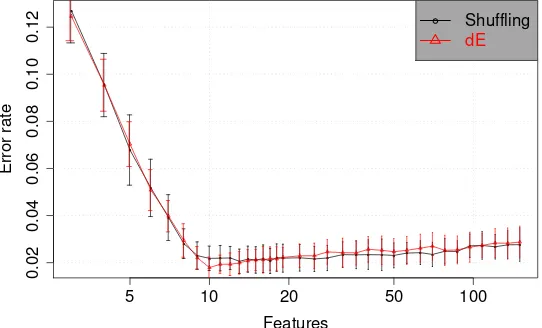
Fig. 1.Mean error rates as a function of the number of variables selected by the ANN-RFE method for the artificial two-Gaussians dataset. Error bars show one standard deviation.
●
●
●
● ●
● ●
● ●●
●●●●●●● ● ● ● ● ● ● ● ● ● ● ● ● ● ● ● ● ● ●
5 10 20 50 100
0.02
0.04
0.06
0.08
0.10
0.12
Features
Error rate
● Shuffling
dE
problem involving two classes, each one sampled from a Gaussian distribution. The problem involves 150 variables, from which 10 are relevant and the remain-ing 140 are uniform noise. In this and all other experiments in this work we used ANNs with a single hidden layer and SOFTMAX outputs [26]. The ANN ensembles were formed with 10 networks in this demonstrative example. The common practice in feature selection is to evaluate the performance of different methods using error curves that shows the resulting average classification error as a function of the number of variables selected. Analyzing results for some fixed number of variables is arbitrary and gives less information, and looking for the minimum error without a bias requires an additional validation set. In Figure 1 we show the classification error levels corresponding to 20 runs of the method. We show the evaluation of both versions of ANN-RFE for a complete selection process, starting with all variables and ending with subsets of 2 variables. The figure indicates that both metrics are very efficient in selecting the 10 relevant variables (dE seems to be slightly more efficient in this case).
3.2 Experimental setup
A feature selection method that uses (in any way) information about the targets may lead to overfitting, in particular with wide datasets. Thus, in order to obtain unbiased estimates of the prediction error, feature ranking and selection should be included in the modeling, and not treated as a pre-processing step; moreover, we need to appropriately decouple selection from error estimation [27].
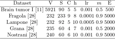
Table 1.Details on the five wide real-world datasets used in this work. Columns show the number of variables (V), samples (S) and classes (C), and the parameters used for
the ANN: hidden units (h), learning rate (lr), momentum (m) and number of epochs
(E).
Dataset V S C h lr m E
Brain tumor I [11] 5921 90 5 5 0.001 0.5 500
Fragola [28] 232 233 9 8 0.0001 0.9 5000
Lampone [28] 232 92 5 10 0.0005 0.9 5000
Grana [28] 235 60 4 7 0.001 0.5 2000
Nostrani [28] 240 60 6 10 0.001 0.9 5000
a random split of the dataset in a training set (used to develop the models – including the feature selection step), and in a test set, used to estimate the ac-curacy of the models. The inner process supports the selection of nested subsets of features and the selection of appropriate parameters and development of clas-sifiers over these subsets (using only the learning subset provided by the outer loop). The results of then= 100 replicated experiments are then aggregated to obtain the accuracy estimation and stability evaluations.
As we stated before, we always use ANNs with a single hidden layer and SOFTMAX outputs [26]. All bagging ensembles have 100 ANN members.
3.3 Datasets
We use five different wide real-world datasets in this work. The first one corre-sponds to gene expression of brain tumor cells, evaluated with DNA microchips. The other four are concentration of volatiles from agro-industrial products, eval-uated with PTR-MS mass-spectrometry. In Table 1 we show some details on the datasets and the original reference for each one. We also show the ANN settings we used in each case.
3.4 Individual ANN vs Ensembles
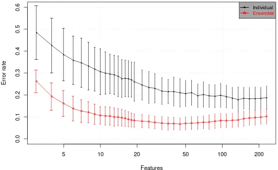
A relevant question at this point is if it is needed to use full ensembles to measure features importance. In Figure 2 we show a comparison between ANN-RFE applied to the Fragola dataset, using an individual ANN and an ensemble of 100 networks. Ensembles produce better classifiers, as is well known from previous works [18, 23] and also better and more stable selections, as follows from the figure. We repeated the experiment with other datasets with the same qualitative results (figures not shown for lack of space).
3.5 Evaluation of the two metrics
Fig. 2.A comparison between selection made with an individual ANN and an ensemble. The figure shows error rates as a function of the number of variables selected by both methods for the Fragola dataset.
● ●
● ●
● ●
● ● ●●●●
●●● ● ●
● ● ●
● ● ● ● ● ●
● ● ● ● ● ● ● ● ● ● ● ● ●
5 10 20 50 100 200
0.0
0.1
0.2
0.3
0.4
0.5
0.6
Features
Error rate
● Individual
Ensemble
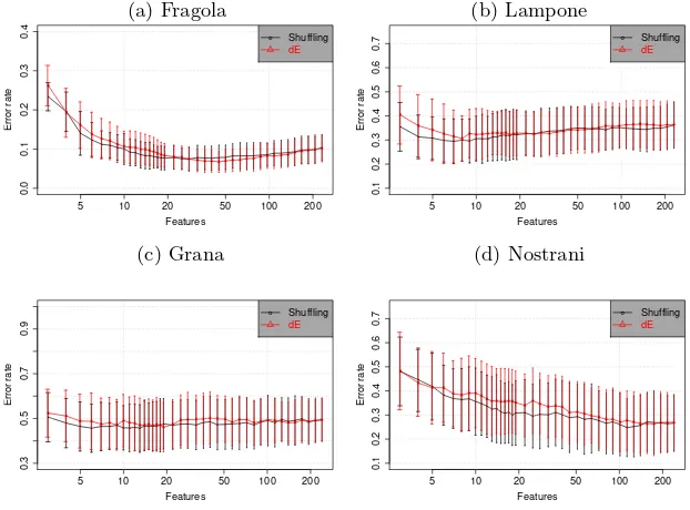
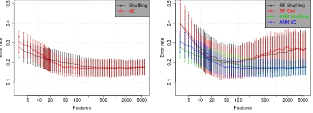
panels, because they are mostly related to the use of very small test sets in some cases. Overall, the shuffling metric shows a slightly better performance, in particular with small features subsets (the most relevant section of these ex-periments). In the left panel of Figure 5 we show the same comparison for the gene-expression dataset.dEshows a better performance in this case, except for subsets with very few features, when error levels have raised considerably.
3.6 Comparison with other relevance measures
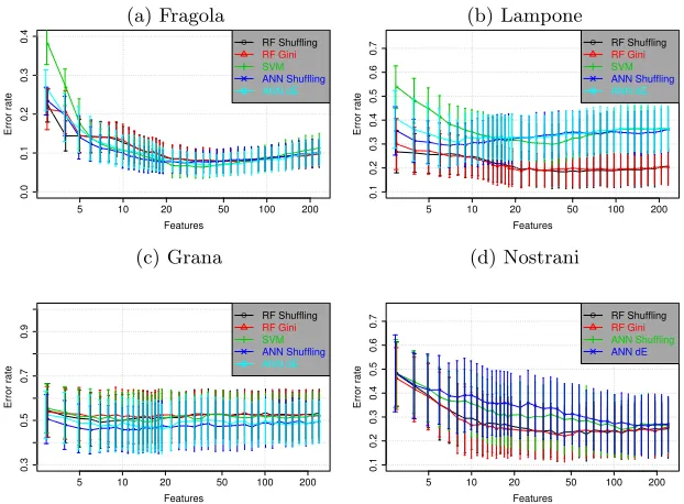
In this last experiment we compared the new ANN-based metrics with three previously used measures for RFE: i) importance extracted from linear SVM [8], ii) from RF measured by shuffling the dataset [14, 13] and iii) from RF averages of the GINI index [14]. We added the RF-GINI measure because it has important similarities with ourdE metric, as it is evaluated directly on the cost function using the training set only, not the OOB sets. In all cases we used the corresponding classifiers after the selection (RF for RF-based methods, SVM for SVM-based selections).
Fig. 3. Comparison of the two metrics introduced in this work for the ANN-RFE method. The figure shows error rates as a function of the number of variables selected by the ANN-RFE method for the PTR-MS datasets.
(a) Fragola (b) Lampone
● ● ● ● ●● ●● ●● ●●●●● ● ●●●●●●●●●●●●●●● ●●●●●●●●
5 10 20 50 100 200
0.0 0.1 0.2 0.3 0.4 Features Error rate ● Shuffling dE ● ● ● ● ●●●●●●●●●●●● ● ●●●●●●●●●●●● ●●●●●●●●● ●
5 10 20 50 100 200
0.1 0.2 0.3 0.4 0.5 0.6 0.7 Features Error rate ● Shuffling dE
(c) Grana (d) Nostrani
● ● ● ●●●●●●●●●●●● ●●●●●●●● ●●●●●● ●● ● ●●●● ●●●
5 10 20 50 100 200
0.3 0.5 0.7 0.9 Features Error rate ● Shuffling dE ● ● ● ● ●●●● ● ● ●● ●●● ● ●● ●●●●● ●●●●● ●● ● ●●● ●●●●●
5 10 20 50 100 200
0.1 0.2 0.3 0.4 0.5 0.6 0.7 Features Error rate ● Shuffling dE
Nostrani dataset RF based methods performs better than ANN-RFE in the feature selection process.
The results of the same comparison on the gene-expression dataset can be analyzed in Figure 5, right panel. This dataset shows the same situation as the Lampone dataset, but inverted. In this case ANN-RFE is always better, but the difference is more related to a better modeling than to a better feature selection.
4
Conclusions
In this paper we have introduced the ANN-RFE, a new technique for feature selection that combines the accurate and time-efficient RFE method with the strong discrimination capabilities of ANN ensembles. We also discussed two fea-ture importance metrics that can be used with ANN-RFE: the shuffling and
dE metrics. After showing the potential of the new method with an artificial dataset, we applied it to five real-world wide datasets.
Fig. 4. Comparison of different selection methods in four PTR-MS datasets. Panels show error rates as a function of the number of selected variables.
(a) Fragola (b) Lampone
●
● ● ● ●●● ●●●
●●●●●●●
●●●●●●●●●●●●●●●●●●●●●●
5 10 20 50 100 200
0.0 0.1 0.2 0.3 0.4 Features Error rate
● RF Shuffling
RF Gini SVM ANN Shuffling ANN dE ● ● ● ● ●●●●●●●●●● ●● ● ●●●●●●●●●●●●●●●●●●●●●●
5 10 20 50 100 200
0.1 0.2 0.3 0.4 0.5 0.6 0.7 Features Error rate
● RF Shuffling
RF Gini SVM ANN Shuffling ANN dE
(c) Grana (d) Nostrani
● ● ● ● ●●●●●●●●● ● ●●●●●● ●●●●●●●●●●●●●●●●●●●
5 10 20 50 100 200
0.3 0.5 0.7 0.9 Features Error rate
● RF Shuffling
RF Gini SVM ANN Shuffling ANN dE ● ● ● ● ● ● ●● ● ●●●●●● ●● ●●●●● ●●●● ● ●●● ● ● ●● ●●●●●
5 10 20 50 100 200
0.1 0.2 0.3 0.4 0.5 0.6 0.7 Features Error rate
● RF Shuffling
RF Gini ANN Shuffling ANN dE
to. When faced with a problem in which ANN ensembles are the best modeling strategy (as the Brain tumors I dataset), it is expected that a feature selection strategy based directly on ANNs should give the best performance.
Several avenues are open to continue this work. Of course, a more in depth evaluation is needed, including more datasets and other aspects of the method, as for example the influence of the number of networks or the degree of over-fitting of the individual members of the ensemble. The stability of the selection [28] also needs research. The dE metric has the advantage of not using at all the OOB datasets, which then could be used to produce unbiased estimates of prediction errors without keeping a test set aside, improving the efficiency of the full selection method.
Acknowledgements
We acknowledge partial support for this project from ANPCyT (grant PICT 643).
References
Fig. 5.Results on the Brain tumors I dataset (error rates as a function of the number of selected variables). Left panel: Comparison of the two metrics introduced in this work for the ANN-RFE method. Right panel: Comparison of ANN-RFE with RF-RFE.
● ● ●● ● ●●● ● ●● ● ● ● ● ●●●●●●●●●●●●●●●● ●● ●●●●●●●●●●●●●●●●●●●●●●●●●●●● ●●●●●●●●●
5 10 20 50 100 500 2000 5000
0.1 0.2 0.3 0.4 0.5 Features Error rate ● Shuffling dE ● ● ● ● ●● ●● ●● ●●●●●● ●●●● ● ● ●●●●●●●●●●● ●●● ●●●●● ●● ●●●●●● ●●●●● ●●●●● ●●●●● ● ●● ● ●●
5 10 20 50 100 500 2000 5000
0.1 0.2 0.3 0.4 0.5 Features Error rate
● RF Shuffling
RF Gini ANN Shuffling ANN dE
2. Guyon, I., Elisseeff, A.: An Introduction to Variable and Feature Selection. J. Mach. Learn. Res. 3, 1157–1182 (2003).
3. Liu, H., Dougherty, E.R., Dy, J.G., Torkkola, K., Tuv, E., Peng, H., Ding, C., Long, F., Berens, M., Parsons, L., Zhao, Z., Yu, Z., Forman, G.: Evolving Feature Selection. IEEE Intelligent Systems, 20:6, 64–76 (2005).
4. Golub, T.R., Slonim, D.K., Tamayo, P., Huard, C., Gaasenbeek, M., Mesirov, J.P., et al., Molecular Classification of Cancer: Class Discovery and Class Prediction by Gene Expression. Science, 286, 531-537 (1999).
5. Li, H., Ung, C. Y., Yap, C. W., Xue, Y., Li, Z. R., Cao, Z. W., Chen Y. Z.: Prediction of Genotoxicity of Chemical Compounds by Statistical Learning Methods. Chem. Res. Toxicol. 18, 1071–1080 (2005).
6. Lindinger, W., Hansel, A., Jordan, A.: On-line monitoring of volatile organic com-pounds at ppt level by means of Proton-Transfer-Reaction Mass Spectrometry (PTR-MS): Medical application, food control and environmental research. Int. J. Mass. Spectrom. Ion Procs. 173, 191-241 (1998).
7. Biasioli, F., Gasperi, F., Aprea, E., Mott, D., Boscaini, E., Mayr, D., M¨ark, T.D.:
Coupling Proton Transfer Reaction-Mass Spectrometry with Linear Discriminant Analysis: a Case Study. J. Agr. Food Chem. 51, 7227-7233 (2003).
8. Guyon, I., Weston, J., Barnhill, S., Vapnik, V.: Gene Selection for Cancer Classifi-cation using Support Vector Machines. Mach. Learn. 46, 389–422 (2002).
9. Vapnik, V.: The Nature of Statistical Learning Theory. Springer, New York (1995). 10. Ramaswamy, S., et al.: Multiclass cancer diagnosis using tumor gene expression
signatures. P. Natl. Acad. Sci. USA 98, 15149–15154 (2001).
11. Statnikov A., Aliferis, C.F., Tsamardinos, I.,Hardin, D., Levy, S.: A comprehensive evaluation of multicategory classification methods for microarray gene expression cancer diagnosis. Bioinformatics, 21:5, 631–643, (2005).
12. Granitto, P.M., Biasioli, F., Gasperi, F., Furlanello, C.: Modeling Sensory Analysis datasets: the case of Italian Cheeses. Proceedings of JAIIO 2005 - The 34th Inter-national Conference of the Argentine Computer Science and Operational Research Society, Rosario, Argentina (2005).
14. Breiman, L.: Random Forests. Mach. Learn. 45, 5–32 (2001).
15. L. I. Kuncheva Combining Pattern Classifiers. Wiley-Interscience, New Jersey,
2004.
16. A. J. C. Sharkey, editor.Combining Artificial Neural Nets. Springer-Verlag,
Lon-don, 1999.
17. S. Geman, E. Bienenstock and R. Doursat. Neural Networks and the Bias/Variance
Dilemma.Neural Computation4:1-58, 1992.
18. L. Breiman. Bagging predictors.Machine Learning24:123-140, 1996.
19. Y. Freund and R. Schapire. A decision-theoretic generalization of on-line learning
and an application to boosting. In Proceedings of the Second European Conference
on Computational Learning Theory, 23-37, 1995.
20. P. M. Granitto, P. F. Verdes and H. A. Ceccatto. Neural Networks Ensembles:
Evaluation of Aggregation algorithms.Artificial Intelligence163:139-162, 2005.
21. B. Rosen. Ensemble learning using decorrelated neural networks.Connection
Sci-ence. Special Issue on Combining Artificial Neural Nets: Ensemble Approaches
8(3&4):373-384, 1996.
22. H. Schwenk and Y. Bengio. Boosting neural networks. Neural Computation
12:1869-1887, 2000.
23. D. Opitz and R. Maclin. Popular Ensemble Methods: An Empirical Study.Journal
of Artificial Intelligence Research, 11:169-198, 1999.
24. Furlanello, C., Serafini, M., Merler, S., Jurman, G.: Entropy-Based Gene Ranking without Selection Bias for the Predictive Classification of Microarray Data. BMC Bioinformatics 4, 54 (2003).
25. Y. LeCun, J.S. Denker and S.A. Solla. Optimal brain damage. In Advances in
neural information processing systems 2, NIPS 1990, 598-605, 1990.
26. C. M. Bishop.Neural Networks for Pattern Recognition. Oxford University Press,
London, 1995.
27. Ambroise, C., McLachlan G.: Selection bias in gene extraction on the basis of microarray gene-expression data. P. Natl. Acad. Sci. USA 99, 6562–6566 (2002). 28. Granitto, P.M., Biasioli, F., Furlanello C., Gasperi, F.: Efficient Feature Selection