International propagation of shocks: an evaluation of contagion effects for some Latin American countries

SERIE DO C UMENTO S DE TRA BA JO

Se p tie m b re 2009

INTERNATIONAL PROPAGATION OF SHOCKS:

AN EVALUATION OF CONTAGION EFFECTS FOR SOME

LATIN AMERICAN COUNTRIES

International propagation of shocks:

An evaluation of contagion effects for some Latin American countries

Manuel Ramírez Constanza Martínez

Universidad del Rosario

Abstract

In this paper we analyze the spread of shocks across assets markets in eight

Latin-American countries. First, we measure the extent of markets reactions

with the Principal Components Analysis. And second, we investigate the

volatility of assets markets based in ARCH-GARCH models in function of the

principal components retained in the first stage. Our results do not support the

existence of financial contagion, but of interdependence in most of the cases

and a slight increase in the sensibility of markets to recent shocks.

JEL: F30, F32, F34

Keywords: assets markets, financial contagion, interdependence

1. Introduction

The international trade, financial markets relations and decisions of investors constitute the

main transmission channels of shocks, because these means imply capital movements

across countries. All shocks: regional or domestic affect the assets markets in different

magnitudes. According to Forbes and Rigobon (2000) if the market’s reaction in a country

after the occurrence of a shock in another country is extreme, that market is experiencing

financial contagion. But if the reaction is smooth and is linked to the evolution of the

macroeconomic fundamentals of that country, is a case of interdependence.

The spread of financial contagion is attributable to the decisions of investors. Once an

countries or markets that under their criteria have not been affected yet; their decisions

contribute, in such a way, to the spread of financial contagion or to the deepening of its

consequences across countries and assets markets.

The transmission of shocks is not related to the level of development of the countries.

However, since the emerging countries seem more sensitive to its effects, the literature has

devoted huge efforts to the understanding of these types of cases. Most of the research in

this line is focused in the consequences of shocks that affected Asian and Latin American

countries, between 1994 and the end of the 90s (Calvo and Reinhart 1996, Rigobon 1999,

Kaminksy and Reinhart 2003, Edwards and Susmel 2001, Hashimoto and Ito 2004). Since

then, several financial events have occurred and have not been explored yet.

In this paper we investigate the assets markets reactions in Argentina, Brazil, Colombia,

Chile, Mexico, Peru, Uruguay and Venezuela to shocks that occurred between the end of

the 90s and September of 2008. However, we do not evaluate the global financial crisis that

emerged in 2007 because the crisis and most of its consequences have not come yet to an

end. That is our period of study starts in 1997 and ends with the Lehman Brother’s collapse.

In order to capture the behaviour of assets markets, we consider daily data of exchange rate,

short term interest rate, equity market returns and sovereign spreads. First, we consider the

effects of shocks to the variability of assets markets by using the Principal Components

Analysis. Second, we investigate the volatility of each market with ARCH-GARCH models

based on the principal components retained in the initial stage. Our results do not support

Besides, we found extreme cases of assets markets isolated of the region trends represented

by Argentina, Uruguay and Venezuela.

The paper proceeds as follows. Section 2 presents the most relevant findings of financial

contagion; Section 3 describes data set and the included exogenous shocks. Section 4

presents the empirical tests and comments on the most important results associated to the

Principal Components Analysis and ARCH –GARCH models. Section 5 concludes.

2. Contagion Empirical Literature

The propagation of shocks across countries and assets markets may end in financial

contagion or in interdependence, according to the extent of the reaction displayed by the

markets. Forbes and Rigobon (2000) affirm that the first case is represented by a significant

increase in cross market linkages after the occurrence of a shock, which can not be

explained by the evolution of the domestic macroeconomic fundamentals. So that, if the

assets market’s reaction is extreme represents financial contagion, but if that reaction is

smooth and is attributable to the economy’s fundamentals, represents interdependence.

The financial contagion is associated to the evaluation of particular events, which in most

cases are related to shocks with perverse effects on economies, such as the currency crises

and government’s debt default (Eichengreen, Rose and Wyplosz 1996, Baig and Goldfajn

1998, 2000, Bazdresch and Werner 2000). Several types of shocks may affect the capital

markets, but the spread of its effects across countries appear from the generalized loss of

and Mendoza (1998) and Agenor and Aizenman (1997) in response to a negative shock, the

investors withdraw their money from the assets markets of the region, without confirming

whether the market where they have invested has been affected or not by that shock.

According to these authors and to Dornbusch, Park and Claessens (2000), investors’

incorrect decisions may induce to irrational movements of capitals, partially attributable to

asymmetries of information and the lack of specific data of the country where they

invested. The decisions of investors may create financial contagion in countries not

infected, or deepen its consequences in countries previously affected by shocks.

Within the type of shocks that conduct to financial contagion, the effects of currency crises

have been widely explored in the empirical literature. The Mexican Tequila effect in 1994,

the Asian currency crisis in 1997, the Russian devaluation in 1998, the Brazilian

devaluation in 1999 and the Turkish devaluation in 2001; and the way in which those

shocks affected other economies have been the centre of research (Eichengreen et al 1996,

Agenor et al 1997, Glick and Rose 1998, Kodres and Pritsker 1999, Rigobon 1999,

Kaminsky and Reinhart 2000a, 2001, Pritsker 2000, Bazdresch and Werner 2000, Forbes et

al 2000, Baig et al 2000, Bordo and Murshid 2000, and Fazio 2007). These studies coincide

in that financial contagion is not a global trend. The propagation of shocks goes from the

infected country toward those economies connected by trade or financial relations.

The financial contagion does not affect all countries in a similar fashion, not even to those

with similar levels of development or economic conditions. In this matter the empirical

literature that has included the role played by restrictions to capitals mobility, has not come

controls policies in the Chilean economy, between 1990s and the end of that decade,

avoided the consequences of Asian contagion and some Latin American crises that affected

other countries in the region. But other studies, including a broad set of countries (De

Gregorio and Valdés (2000) and Kaminsky et al (2001)) and specifically for Colombia

(Concha, Galindo and Quevedo, 2008) suggest that capital controls did not stop the

appreciation of the domestic currency and the foreign capital inflows in the end of 90’s.

3. Data and Financial events to be tested

We use daily data of four assets market variables. The first variable is the exchange rate

which accounts for the economy’s strength related to other countries and is measured by the

percentage changes of domestic currency per U.S dollar. For the money market we include

the short term interest rate, represented by the overnight interbank interest rate (in most of

the countries) in order to capture the domestic monetary policy. In third place we analyze

the equities returns on assets markets by calculating the percentage changes of the stock

market index per country. And finally, we include the sovereign bond spreads represented

by the Emerging Market Bond Index (EMBI), to analyze the perceived risk among

international investors. This index represents the excess of return related to the U.S treasury

bonds that emerging countries should offer when trading its debt in international markets.

Our sample is composed by seven Latin-American countries, with data from January 1st of

1997 to September 30th of 2008, but with small differences in the availability of

information per markets. In holidays and banking days we include the same data registered

countries we include are Argentina, Brazil, Chile, Colombia, Mexico, Peru, Venezuela and

Uruguay. For this last country the only information available were the exchange rate and

the overnight interbank interest rate. Other countries such as Panama and Dominican

Republic were excluded, because of the lack of a formal Stock Exchange Market and the

adoption of the U.S dollar as the domestic currency. For this last reason, we also exclude

Ecuador, besides the fact that this country does not report data of short term interest rate.

The tests of the spread of shocks among countries are based on four negative financial

episodes and four positives. The negatives are: NASDAQ crisis, Turkish devaluation,

Argentinean devaluation and sovereign debt default, and the Brazilian confidence crisis in

2002. The positives shocks are the debt’s upgrade of Mexico, Colombia, Peru and Brazil.

We do not include other events previous to the mentioned above, like: the Mexican Tequila

effect, Russian debt default, Asian crisis, and Brazilian devaluation, because Colombian

data on equity markets and sovereign spreads are not available for that period. The data of

Colombian stock market prior to July of 2001 depend on three markets indexes for the

biggest cities (Bogotá, Medellin and Cali). Each market index is composed by different

assets baskets and reflects differences in the volumes traded; and that do not allow us to

construct a single index for the country. In relation to the variable that captures Colombian

sovereign risk, the data of EMBI are not available before December 31st of 19971.

In order to provide information related to the shocks, we summarize the events as follows:

1

• Nasdaq crisis in April 2000: this index reflects the evolution of equities associated

to the internet, telecommunications and computer software and hardware. As

summarized by Johansen and Sornette (2000) in the spring season of 1997 this

index experienced a speculative bubble, as a result of the generalized expectations

of increasing future earnings, and not by the strengthening of the U.S economic

fundamentals. The Nasdaq crisis exploded three years later, in the mid of April of

2000, when the index lost around 40% of its market value.

• Turkish devaluation: By the end of the 90’s the monetary indicators of this country

were characterized by a high interest rates and high inflation. The monetary

authorities, with the purpose to control this situation, adopted a fixed exchange rate

in December of 1999. However, since the exchange rate value at which the

domestic currency was tied to the U.S dollar was overestimated, the productive

sector had to face huge increases in the costs of inputs. As a result, the economy

suffered a strong fall in the total exports that induced to an increase in the deficit of

the balance of payments. That deficit was also enlarged by the outflows of foreign

capitals that the country underwent since the year 2000. The final outcome: a 30%

depreciation of the Turkish lira’s in February 22 of 2001 (Hristov, 2002).

• Argentinean debt default and devaluation: Before the end of the 90's the

government pushed the banks and retirement funds to buy and maintain papers of

public debt denominated in US currency, in order to finance its expenditure. But the

management started to mine the economy’s stability in 2001. The generalized loss

of confidence in the economy generated a massive withdrawal of savings and funds

of the financial system that accounted for a 20% fall of total deposits during that

year. The situation became even more complex in November of 2001 with the

liquidity restrictions adopted by the government, such as: i) the restriction of the

monthly withdrawals to a maximum of US$1,000 per client; ii) the change of the

sovereign debt papers previously acquired by banks, with papers with no liquidity,

so that their value became a direct credit to the government; iii) the imposition of

ceilings to the deposits interest rates. The economic instability was magnified by the

declaration of debt default in the end of December of 2001, and deepened a month

later when the government devaluated its domestic currency in 290% (CLAF 2002).

• Confidence crisis in Brazil (Mineiro 2002): During 1994 the government adopted

some economic measures with the purpose of liberalize the trade and financial

relations. These policies were based in the increase of domestic investment and

public expenditure mostly financed with foreign capitals inflows. The economy

worked reasonably well until 1998, right after the liquidity problems emerged in

response to a strong capital outflows. The situation worsened in January of 1999

since the country was forced to conduct a strong devaluation of its domestic

currency (the Real); and became even critical by the end of 2001, when its main

trade partner: Argentina, did enter in debt default. During these years the economy

exhibited an increasing internal and external debt that continued to grow, reaching

60% of GDP in July of 2002. Almost 30% of the public debt was tied to the US

In July of 2002 the confidence crisis emerged, also augmented by the dominance of

the candidate Lula Da Silva in the presidential elections.

• Debts ratings upgrades: the Mexican debt was elevated by Moody’s agency to the

investment grade in March 7th of 2000. The Colombian and Brazilian debt were

taken to the BBB- level by Standard and Poor’s (which corresponds to investment

grade), in June 12 of 2007 and April 30 of 2008, respectively. The Peruvian credit

rating was also upgraded in April 2 of 2008 by the Fitch Agency.

4. Empirical tests

Our empirical tests for financial contagion consist of two procedures. We first investigate

the evolution of assets markets with the Principal Components Analysis (PCA) for the

entire sample and for each sample in the eight financial episodes. For these

sub-samples we define periods before and after shocks, omitting the time during which each

one took place. Otherwise, our results could incorrectly determine the existence of financial

contagion. In a second stage we analyze the volatility of markets based in ARCH-GARCH

models, obtained from the PCA's retained components.

Before conducting PCA we standardized all variables in order to prevent that differences in

the variances of the series generate distortions in our results (Kaminsky et al 2001

employed the same standardization, ensuring that all variables have zero mean and unit

standard deviation). Therefore we confirm that the PCA is a suitable method to study the

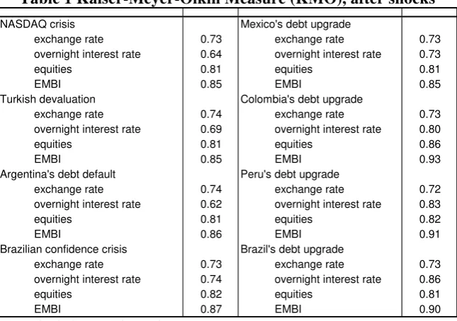
an index that compares the magnitudes of the observed correlation coefficients with the

partial correlation coefficients. The higher the result of this statistic the stronger is the

relationship of assets markets among countries.

Table 1 Kaiser-Meyer-Olkin Measure (KMO), after shocks

NASDAQ crisis Mexico's debt upgrade

exchange rate 0.73 exchange rate 0.73

overnight interest rate 0.64 overnight interest rate 0.73

equities 0.81 equities 0.81

EMBI 0.85 EMBI 0.85

Turkish devaluation Colombia's debt upgrade

exchange rate 0.74 exchange rate 0.73

overnight interest rate 0.69 overnight interest rate 0.80

equities 0.81 equities 0.86

EMBI 0.85 EMBI 0.93

Argentina's debt default Peru's debt upgrade

exchange rate 0.74 exchange rate 0.72

overnight interest rate 0.62 overnight interest rate 0.83

equities 0.81 equities 0.82

EMBI 0.86 EMBI 0.91

Brazilian confidence crisis Brazil's debt upgrade

exchange rate 0.73 exchange rate 0.73

overnight interest rate 0.74 overnight interest rate 0.86

equities 0.82 equities 0.81

EMBI 0.87 EMBI 0.90

Calculations of the authors

Our results of KMO in Table 1 validate the PCA procedure with statistics that surpass the

critical bound of 0.60, required to consistently apply this procedure. In other words, the

markets reactions of these Latin-American countries after shocks are closely connected.

a. Principal components analysis (PCA)

The PCA is a method of data reduction that is linear in variables and produces a smaller

number of new non-correlated variables that explain most of the original series variances.

The procedure consists in the decomposition of the series into its vectors and

absolute value represent the strength of co-movement of each country with respect to other

Latin-American countries (LAC).

In the study of assets markets behaviour the first principal component can be considered as

indicator of regional risk because it measures the degree of common movement displayed

by markets. In such a way, the percentage of variance explained by this component

measures the markets' reaction after shocks. According to Fuentes and Godoy (2005) if the

percentage of variance surpasses 50% the assets markets are displaying an extreme

coupling, suggesting financial contagion. A lower reaction, in between 35-50%,

corresponds to markets with a strong coupling, which support the existence of

interdependence. And percentages below 35% imply a weak coupling, a common result of

markets disconnected of the regional trends.

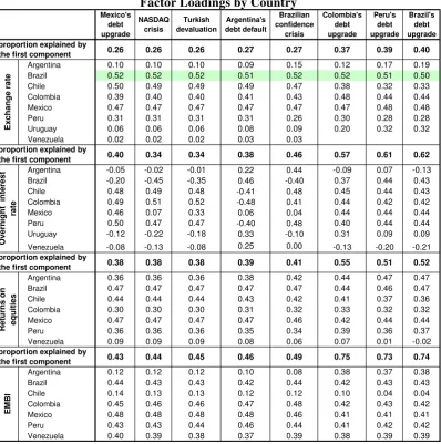
Our results identify differences in the consequences of shocks among countries and assets

markets (Table 2). From the thresholds proposed by Fuentes and Godoy (2005) we

recognize few cases of extreme coupling but not very conclusive in relation to the existence

of contagion. The majority of our eigen-vectors suggest that assets markets co-movements

reflect interdependence; and few specific results display no transmission of shocks at all.

In the exchange rate market the largest extent of co-movement is explained by Brazil, with

factor loadings that surpass 0.50 in all events, however percentages are not far from the

middle threshold. These results of Brazil are slightly followed by Mexico, Chile and

Colombia. But, the Chilean exchange rate increases only after the occurrence of negative

These differences should be taken carefully, since in all countries the government sudden

interventions impede that domestic currencies freely float, and this fact may bias the tests

of exchange rates. Some severe cases of this type of interventions are represented by

Argentina and Venezuela, with currencies that have been fixed to the U.S dollar. Our

results confirm this situation, with a very low proportion of the variance explained by the

first component for both countries. At least for the domestic currencies markets, the factor

loadings results do not support the existence of financial contagion, but of interdependence.

In relation to the short term interest rate the greatest extent of co-movement is presented by

Chile, Colombia and Peru; an outcome that may be attributable to similarities in: its short

term monetary policy or the foreign capitals inflows trends that each country receives. In

either of these alternatives the money markets responses to shocks (though high) only

reflects interdependence. In the other extreme we found the Argentinean and Venezuelan

interest rates, with factor loadings very close to zero. In such a way, the exchange rate

results along with the overnight interest rate suggest that the markets of both countries are

not correlated with the other countries of the region.

In the markets of equities we distinguish two different types: strong coupling markets

(evidencing interdependence) and markets isolated of the region's trends. In the first

category we found Brazil, Chile and Mexico as the markets that display the highest extent

of reaction to shocks: positives or negatives. At least for the case of Brazil this outcome

could be associated with a foreign portfolio investment in equities that averaged an increase

of 145.9% between 2002 and 2006, according to the IMF statistics. Argentina follows the

recent positive shocks. In the second group we found the markets of Colombia and

Venezuela. The factor loadings of Colombian stocks exchange display weak couplings with

the rest of LAC. Calvo and Reinhart (1996) found the same result for this country and that

is very intuitive since the behaviour of this market mostly depends on the decisions of

domestic investors. The Venezuelan case exhibited the lowest factor loadings of the group

which imply that the international shocks do not generate large effects in this market.

Table 2 Principal Components Analysis after shocks Factor Loadings by Country

0.26 0.26 0.26 0.27 0.27 0.37 0.39 0.40

Argentina 0.10 0.10 0.10 0.09 0.15 0.12 0.17 0.19

Brazil 0.52 0.52 0.52 0.51 0.52 0.52 0.51 0.50

Chile 0.50 0.49 0.49 0.49 0.47 0.38 0.32 0.33

Colombia 0.39 0.40 0.40 0.41 0.43 0.48 0.44 0.44

Mexico 0.47 0.47 0.47 0.47 0.47 0.47 0.48 0.48

Peru 0.31 0.31 0.31 0.31 0.26 0.30 0.28 0.28

Uruguay 0.06 0.06 0.06 0.08 0.09 0.20 0.32 0.32

Venezuela 0.02 0.02 0.02 0.03 0.03

0.40 0.34 0.34 0.38 0.46 0.57 0.61 0.62

Argentina -0.05 -0.02 -0.01 0.22 0.44 -0.09 0.07 -0.13

Brazil -0.20 -0.45 -0.35 0.46 -0.40 0.37 0.44 0.43

Chile 0.48 0.49 0.48 -0.41 0.48 0.45 0.44 0.43

Colombia 0.49 0.51 0.52 -0.48 0.41 0.44 0.42 0.42

Mexico 0.46 0.07 0.33 0.06 0.04 0.44 0.44 0.44

Peru 0.50 0.47 0.47 -0.40 0.48 0.40 0.44 0.44

Uruguay -0.12 -0.22 -0.18 0.33 -0.10 0.31 0.09 0.09

Venezuela -0.08 -0.13 -0.08 0.25 0.00 -0.13 -0.20 -0.21

0.38 0.38 0.38 0.39 0.41 0.55 0.51 0.52

Argentina 0.36 0.36 0.36 0.38 0.42 0.44 0.47 0.47

Brazil 0.47 0.47 0.47 0.47 0.47 0.44 0.46 0.47

Chile 0.44 0.44 0.44 0.43 0.42 0.41 0.37 0.36

Colombia 0.30 0.30 0.30 0.31 0.32 0.33 0.32 0.32

Mexico 0.47 0.47 0.47 0.47 0.46 0.42 0.44 0.44

Peru 0.36 0.36 0.36 0.35 0.34 0.39 0.36 0.37

Venezuela 0.09 0.09 0.09 0.08 0.06 0.07 0.01 -0.02

0.43 0.44 0.45 0.46 0.49 0.75 0.73 0.74

Argentina 0.12 0.12 0.12 0.10 0.08 0.38 0.37 0.38

Brazil 0.44 0.43 0.43 0.42 0.44 0.42 0.43 0.43

Chile 0.14 0.13 0.13 0.12 0.12 0.10 0.04 0.04

Colombia 0.45 0.46 0.46 0.47 0.48 0.42 0.43 0.42

Mexico 0.48 0.48 0.48 0.48 0.46 0.41 0.41 0.41

Peru 0.43 0.43 0.44 0.46 0.44 0.41 0.42 0.42

Venezuela 0.40 0.39 0.38 0.37 0.39 0.38 0.39 0.39

proportion explained by the first component

EM B I O v e rnight intere s t rat e

proportion explained by the first component

Re tu rn s o n eq uities E x ch an g e r at e

proportion explained by the first component

proportion explained by the first component

Peru's debt upgrade Brazil's debt upgrade Argentina's debt default Turkish devaluation NASDAQ crisis Mexico's debt upgrade Colombia's debt upgrade Brazilian confidence crisis

The sovereign debt spreads exhibit small reactions to the shocks evaluated. With exception

of Chile, the remaining countries evidence strong coupling with factor loadings that vary

among 0.40 and 0.48 which point interdependence. The responses of Colombia, Mexico

and Peru are stronger after a negative shock, suggesting a higher sensibility to bad news. In

the other extreme is Chile, a country that displays the lowest sovereign risk, in contrast to

the other countries in the sample. For this outcome we propose two explanations. First,

foreign investment in Chile is more stable than that registered in other LAC. And second,

the stability and faultless management that the Chilean government has made of its

domestic public debt. Recently, the Standard and Poor’s agency conferred the (AA+) rating,

which corresponds to a country with very strong capacity to repay its sovereign debt.

In the graphs below we present the proportion explained by the first two principal

components per assets market. For more recent shocks, especially for those that occurred

after the beginning of 2000, the sensibility displayed by the first principal component is

increasing and rapidly approximate to the limit of extreme coupling. However, the assets

markets reactions also coincide with shocks originated in the Latin-American region.

Graphs 1 Assets markets sensibility to shocks

(Proportion explained by each component)

Exchange rate 0.0 0.2 0.4 0.6 0.8 1.0 M e xi co 's up gr a de N A SD AQ c ris is Tu rk is h de v a lu at io n A rge nti n a' s de bt de fa ul t Br a z ilia n co n fid e n c e c ris is Co lo m b ia 's up gr a de Pe ru 's up gr a de Br a z il' s up gr a de

Component 1 Component 2

Overnight interest rate

0.0 0.2 0.4 0.6 0.8 1.0 M e xi co 's up gr a de N ASD AQ c ris is Tu rk is h dev al ua tio n A rge nt ina 's de bt de fau lt B raz ili an co n fid e n c e cr isi s C o lo m b ia 's up gr a de Pe ru 's up gr ad e Br a z il' s up gr ad e

Equities 0.0 0.2 0.4 0.6 0.8 1.0 M e xi co 's up gr a de NA S DA Q c ris is Tu rk is h de v a lu at ion A rge nti n a 's de bt de fau lt B ra z ilia n c o nfi d en c e c ris is C o lo m b ia 's up gr a de Pe ru 's up gr a de Br a z il' s up gr a de

Component 1 Component 2

Sovereing bond spreads

0.0 0.2 0.4 0.6 0.8 1.0 M e xi co 's up gr ad e N ASD AQ cr is is Tu rk is h d ev al uat io n A rge nt ina 's de bt def au lt Br a z ilia n c o nf id enc e c ris is C o lo m b ia 's up gr ad e Pe ru 's up gr a de Br a z il' s up gr a de

Component 1 Component 2

Calculations of the authors

Even though the equity markets and exchange rates display a slight increase in the

sensibility to shocks, our results support the existence of interdependence in all period. The

short term interest rate and the sovereign debt spreads have also been linked to their region

counterparts by interdependence. However, both markets have been experiencing increases

in the sensibility, especially as response to positive and recent shocks.

b. ARCH and GARCH models

In this stage we calculate the volatility models with the components retained from the PCA

procedure. These models are appropriate to study the dynamics of assets markets because

allow us to remove the excess of kurtosis present in most of our data. Besides, as suggested

by Forbes and Rigobon (2000), evaluations of financial contagion with traditional tests in

presence of heteroscedasticity may generate biased results in favour of financial contagion2.

2

According to Bollerslev (1990) the formal representation for a GARCH(1,1) is given by:

(2)

(1)

2 1 2

1 2

1

− −

= −

+ +

=

+

=

∑

t t

t k

i

t i t i t

c r r

βσ αε

σ

ε γ

In the equation (1) r_t is the jth principal component obtained in the first stage, which also

denotes the returns of the assets market and the second term (ε_t) is the conditional mean

residual of random shocks. The equation (2) represents the conditional variance of stock

returns over time.

Our results fulfil the necessary condition to correctly analyze the volatility spreads among

markets, which is that the standardized residuals are not serially correlated. In the last

column of Table 3 we present the results for this ARCH test3.

Concerning to the conditional variance equation, the alpha (α) coefficients measure the

extent of reaction to shocks while the bethas (β) capture the persistence of volatility. Per

type of markets, the calculated alphas suggest that the overnight interest rates exhibit a

marked strong reaction to shocks. Our estimators for Argentina, Colombia, Mexico and

Peru exceeded the unity, while for Brazil and Chile these coefficients tended to 0.6.

However, the persistence in volatility for all of these markets is extremely low implying

that the effects of shocks on the assets markets eventually disappear.

3

Table 3 Volatility Spillover among Latin-American assets markets Coefficient p-value

Constant 0.00 0.00

α 0.03 0.00

β 0.95 0.00

Constant 0.00 0.00

α1 0.21 0.00

α2 -0.12 0.00

β 0.90 0.00

Constant 0.00 0.00

α 0.06 0.00

β 0.92 0.00

Constant 0.00 0.00

α 0.14 0.00

β 0.85 0.00

Constant 0.00 0.00

α 0.08 0.00

β 0.88 0.00

Constant

α1 0.21 0.00

α2 -0.12 0.00

β 0.91 0.00

Constant 0.00 0.00

α 0.11 0.00

β 0.89 0.00

Constant

α 0.01 0.00

β 0.99 0.00

Exchange rate market

Brazil

Principal Component 1

Argentina ARCH-test (Probability) Colombia Chile Peru Mexico Venezuela IGARCH 0.771 0.979 0.696 Uruguay 0.806 0.970 0.140 0.053 0.864 Coefficient p-value

Constant 0.000 0.000

α 1.203 0.000

Constant 0.000 0.205

α 0.580 0.000

β 0.483 0.000

Constant 0.000 0.000

α 0.592 0.000

β 0.512 0.000

Constant 0.000 0.000

α 1.145 0.000

Constant 0.000 0.000

α 1.151 0.000

Constant 0.000 0.000

α 1.011 0.000

Constant

α 0.088 0.000

β 0.912 0.000

Constant

α1 0.692 0.000

α2 -0.674 0.000

β 0.982 0.000

Overnight interest rates

0.890 ARCH-test (Probability) 0.688 0.102 0.696 0.971 0.238 0.085 0.860 Colombia Brazil

Principal Component 1

Chile Venezuela Argentina Mexico Peru Uruguay

Table 3 Volatility Spillover among Latin-American assets markets (continuation) Coefficient p-value

Constant 0.00 0.00

α 0.07 0.00

β 0.93 0.00

Constant 0.00 0.00

α 0.09 0.00

β 0.85 0.00

Constant 0.00 0.00

α 0.13 0.00

β 0.79 0.00

Constant 0.00 0.00

α 0.21 0.00

β 0.59 0.00

Constant 0.00 0.00

α 0.08 0.00

β 0.84 0.00

Constant 0.00 0.00

α 0.26 0.00

β 0.67 0.00

Constant 0.00 0.00

α 0.19 0.00

β 0.62 0.00

0.625

0.953

Principal Component 1 ARCH-test (Probability)

Brazil Argentina

Chile

Peru

Venezuela 0.901

0.661

0.236

Returns on Equities

0.140

0.892

Mexico Colombia

Coefficient p-value

Constant 0.000 0.001

α1 0.543 0.000

α2 -0.364 0.000

β 0.879 0.000

Constant 0.000 0.000

α1 0.212 0.000

α2 -0.147 0.000

β 0.937 0.000

Constant 0.002 0.000

α 0.499 0.000

Constant 0.000 0.000

α1 0.116 0.000

α2 -0.041 0.028

β 0.925 0.000

Constant 0.001 0.000

α1 0.582 0.000

Constant 0.004 0.000

α 0.417 0.000

Constant 0.007 0.000

α 0.728 0.000

Sovereign risk (EMBI)

Principal Component 1 ARCH-test (Probability)

Venezuela Colombia

0.445 0.918

0.093

0.541

Peru

0.586

0.967

0.964

Chile

Mexico Brazil Argentina

We also carry out a similar analysis for the remaining markets and it produced the opposite

result: a small reaction to shocks with high volatility persistence. Some examples are

provided by the stock exchange markets of Argentina, Brazil, Chile and Mexico, which

imply that the effects of shocks are weak but may generate long lasting consequences.

Per type of shocks, we found differences in the assets markets sensibility to specific shocks.

Following the same methodology used by Kaminsky et al (2002) we classify the dates with

the highest increase in the conditional variance (graphs in the appendix). Our results point

that the turbulences in the markets were stronger after the Brazilian devaluation (in January

13 of 1999) and the Argentinean debt default (in the second half of 2001). The first of these

shocks affected the equity markets of Argentina, Brazil, Colombia, Mexico and Venezuela.

Whereas the second altered the sovereign bond spreads of Argentina, Chile, Colombia and

Mexico, the Mexican exchange rate and the interbank interest rate of Argentina and Peru.

Concerning to the remaining shocks we identify a moderate reaction of Colombia, Mexico

and Brazil’s in 2002 that coincides with the Brazilian confidence crisis that ended with the

election of President Lula.

Our results also reveal that the sensibility to shocks vary from market to market,

presumably by differences in the liquidity and the type of investors that acquire the assets.

In this outcome we coincide with Kaminsky et al (2001) in that the assets markets are not

equally affected by shocks. If assets markets are more open and attract huge amounts of

foreign capitals, its sensibility to shocks should be higher. But if markets mainly depend on

International Monetary Fund, the foreign portfolio investment in equities between 2001 and

2008 reached a cumulative average as percentage of GDP in 2008 of 0.55% in Argentina,

2.69% in Brazil, 2.03% in Chile, 0.34% in Colombia, (-0.04%) in Mexico, 1.51% in Peru

and 0.03% in Venezuela. The Brazilian equity market which was the main receptor of

foreign capitals in Latin America, is precisely the market that exhibit the strongest reactions

to different sorts of shocks. The opposite occurs in Argentina which equity market barely

responds to shocks.

Our results suggest that the markets display higher sensibility to positive and recent shocks.

We identify strong market’s reactions in most of Latin American countries in response to

the debt’s upgrade of Colombia, Peru and Brazil. Besides, we found stronger reactions to

shocks originated regionally in contrast to shocks coming from non Latin-American

countries. For example, the effects of the Turkish’s devaluation were not significant as

shown by our outcomes.

5. Conclusions

The international transmission of shocks across countries ends in financial contagion if the

assets markets reaction is extreme and can not be associated to the fundamentals of the

economy. The spread and consequences of this financial phenomenon are tied to the

decisions of international investors which may be wrong, if asymmetries of information

Our two step procedure for testing the transmission of shocks clearly identifies the

existence of interdependence across assets markets in Latin American countries. Per type of

markets there is no conclusive evidence of financial contagion, however the sensibility to

shocks have been increasing, especially in the cases of the interbank overnight interest rate

and sovereign bond spreads; and also in response to the occurrence of positives and recent

shocks originated in Latin American countries.

We found few cases but not very conclusive of the existence of financial contagion, mostly

related to the exchange rate behaviour in Brazil. We also found that the exchange rates and

overnight interest rates of Argentina, Uruguay and Venezuela are not related to the regional

trends so that their markets reactions to shocks are negligible. Per type of markets the

volatility models suggest small reactions to shocks with high persistence in the assets

markets of the exchange rate, sovereign bonds spreads and stock exchanges.

References

Agénor P., and Aizenman J., (1997) “Contagion and volatility with imperfect credit markets” NBER Working Paper No. 6080

Baccheta P., and Wincoop E., (1998) “Capital Flows to Emerging Markets: Liberalization, Overshooting and Volatility” NBER Working Paper No. 6530

Baig T. and Goldfajn I. (2000) “The Russian Default and the Contagion to Brazil” IMF Working Paper No. 160

Bordo M., and Murshid A., (2000) “Are financial crisis becoming increasingly more contagious? What is the Historical Evidence of Contagion?” World Bank Publication: International Financial Contagion: How it spreads and how it can be stopped

Calvo S., and Reinhart C., (1996) “Capital Flows to Latin America: is there any evidence of Contagion Effects” Munich Personal RePEC Archive

CLAF -Comité Latinoamericano de Asuntos Financieros (2002) “Como resolver la crisis financiera de la Argentina” Declaración número 5

De Gregorio and Valdés (2000) “Crisis transmission: Evidence from the debt, Tequila and Asian Flu crisis” World Bank Publication: International Financial Contagion: How it spreads and how it can be stopped

Dornbusch R. and Claessens S., (2000) “Contagion: how it spreads, and how it can be stopped”, in: International Financial Contagion, World Bank

Edwards S., and Susmel R., (2001) “Volatility Dependence and Contagion in Emerging Equity Markets” NBER Working Paper No. 8506

Fazio G., (2007) “Extreme interdependence and extreme contagion between emerging markets” Journal of International Money and Finance No. 26 pp. 1261-1291

Forbes K, and Rigobon R (1999)a “Measuring Contagion: conceptual and empirical issues”,

in: International Financial Contagion, World Bank

Forbes K, and Rigobon R (1999)b “No contagion, only interdependence: measuring stock

markets co-movements”NBER Working Paper No. 7267

Forbes K, and Rigobon R (2000) “Contagion in Latin America: definitions, measurement and policy implications”

Fuentes M, and Godoy S., (2005) “Sovereign spreads in emerging markets: a principal components analysis” Documento de Trabajo No. 333, Banco Central de Chile

Hashimoto Y., and Ito T., (2004) “High Frequency Contagion between the Exchange Rate and Stock Prices” NBER Working Paper No. 10448

Hernández L., and Valdés R., (2001) “What drives Contagion: Trade, Neighbourhood or Financial Links” IMF Working Paper

Hristov S., (2002) “The Crisis in Turkey” Institute for Regional and International Studies

Johansen and Sornette (2000) “The Nasdaq Crash of April 2000: Yet another example of log-periodicity in a speculative bubble ending in a crash” The European Physical Journal

Kaminsky G., and Reinhart C., (2000)a “On crisis, Contagion and Confusion” Journal of

Kaminsky G., and Reinhart C., (2001) “Financial crises in time of stress” NBER Working Paper Series No. 8569

Kaminsky G., Reinhart C., and Végh (2002) “Two Hundred Years of Contagion”

Kaminsky G., Reinhart C., (2003) “The Centre and the Periphery: The globalization of financial turmoil” NBER Working Paper No. 9479

Lozano I., (2005) “Cálculo y determinantes del componente idiosincrático del spread colombiano” mimeo.

Mineiro A (2002) “Brazil: the real roots of crisis” in Third World Resurgence magazine, issue N 143-144

Park Y., and Song Ch., (2000) “Financial Contagion in the East Asian Crisis- with special reference to the Republic of Korea” World Bank Publication: International Financial Contagion: How it spreads and how it can be stopped

Pesaran H., and Pick A., (2004) “Econometric Issues in the Analysis of Contagion” CESifo Working Paper No. 1176

Pritsker M., (2000) “The Channels for financial contagion” Working Paper, Federal Reserve Board, Washington

Rigobon R. (1999) “On the measurement of international propagation of shocks”, NBER Working Paper 7354

Rigobon R., (2001) “Contagion: How to measure it? NBER Working Paper No. 8118

Appendix- Conditional Variance of Exchange rate returns Argenti n a .000 .001 .002 .003 .004 .005 .006 .007

01 02 03 04 05 06 07 08 Conditional variance Braz il .0000 .0004 .0008 .0012 .0016 .0020 .0024

99 00 01 02 03 04 05 06 07 08 Conditional variance Chi le .00000 .00001 .00002 .00003 .00004 .00005 .00006 .00007 .00008

99 00 01 02 03 04 05 06 07 08 Conditional variance Col o m b ia .0000 .0001 .0002 .0003 .0004 .0005

99 00 01 02 03 04 05 06 07 08 Conditional variance Me xi c o .00000 .00002 .00004 .00006 .00008 .00010 .00012 .00014

99 00 01 02 03 04 05 06 07 08 Conditional variance Pe ru .00000 .00002 .00004 .00006 .00008 .00010 .00012

99 00 01 02 03 04 05 06 07 08 Conditional variance U ru gua y .0000 .0004 .0008 .0012 .0016 .0020 .0024

99 00 01 02 03 04 05 06 07 08 Conditional variance Venezue la .0000 .0001 .0002 .0003 .0004 .0005 .0006 .0007 .0008 .0009

Appendix- Conditional Variance of Short term interest rate A r ge ntina 0 2 4 6 8 10 12 14

97 98 99 00 01 02 03 04 05 06 07 08 Conditional variance Br a z il .00 .01 .02 .03 .04 .05 .06

97 98 99 00 01 02 03 04 05 06 07 08 Conditional variance Chil e .0000 .0001 .0002 .0003 .0004 .0005 .0006 .0007

97 98 99 00 01 02 03 04 05 06 07 08 Conditional variance C o lo mb ia .00 .02 .04 .06 .08 .10 .12

97 98 99 00 01 02 03 04 05 06 07 08 Conditional variance Me xico .00 .01 .02 .03 .04 .05 .06

97 98 99 00 01 02 03 04 05 06 07 08 Conditional variance Peru .00 .05 .10 .15 .20 .25 .30

97 98 99 00 01 02 03 04 05 06 07 08 Conditional variance U rug u ay 0 1 2 3 4 5

97 98 99 00 01 02 03 04 05 06 07 08 Conditional variance Ven ezu ela 0.0 0.2 0.4 0.6 0.8 1.0 1.2

Appendix- Conditional Variance of Stock market returns Arg enti n a .0000 .0004 .0008 .0012 .0016 .0020 .0024 .0028 .0032

01 02 03 04 05 06 07 08 Conditional variance Brazil .0000 .0001 .0002 .0003 .0004 .0005 .0006 .0007

01 02 03 04 05 06 07 08 Conditional variance Ch ile .00000 .00005 .00010 .00015 .00020 .00025 .00030

01 02 03 04 05 06 07 08 Conditional variance Colombia .000 .001 .002 .003 .004 .005 .006

01 02 03 04 05 06 07 08 Conditional variance Mexico .00000 .00004 .00008 .00012 .00016 .00020 .00024 .00028

01 02 03 04 05 06 07 08 Conditional variance Per u .0000 .0004 .0008 .0012 .0016 .0020 .0024 .0028

01 02 03 04 05 06 07 08 Conditional variance Ven ezu el a .000 .001 .002 .003 .004 .005 .006 .007 .008

Appendix- Conditional Variance of Sovereign Bond Spreads Arg e nti n a 0 10 20 30 40 50

99 00 01 02 03 04 05 06 07 08 Conditional variance Brazil 0.0 0.4 0.8 1.2 1.6 2.0

99 00 01 02 03 04 05 06 07 08 Conditional variance Chi le .00 .02 .04 .06 .08 .10 .12 .14 .16

99 00 01 02 03 04 05 06 07 08 Conditional variance Colom b ia .00 .02 .04 .06 .08 .10 .12 .14

99 00 01 02 03 04 05 06 07 08 Conditional variance Me xico .00 .01 .02 .03 .04 .05 .06

99 00 01 02 03 04 05 06 07 08 Conditional variance Peru .00 .04 .08 .12 .16 .20 .24 .28 .32

99 00 01 02 03 04 05 06 07 08 Conditional variance Ven e zu ela 0.0 0.4 0.8 1.2 1.6 2.0 2.4