Essays on political and public economics

Essays on Political and Public Economics

Oskar Nupia

Economics and Business Department

Universitat Pompeu Fabra

Barcelona

Dipòsit legal: B.42902-2007

Contents

Introduction ………. 1

Chapter I Conflict and Wealth ……… 3

Chapter II Decentralization, Corruption and Political Accountability in

Developing Countries ………. 32

Chapter III Bargaining in Legislatures:

Does the Number of Parties Matter? ………... 60

Acknowledgment

Introduction

This thesis deals with three issues related to public and political economics: (1) The effect of income distribution on conflict; (2) the effect of decentralization on corruption in the presence of powerful local elites; and (3) the effect of the number of parties on the negotiation outcomes in a legislature. To study these relationships is useful to understand several situations that involve collective actions, elite behaviors, and bargaining processes. Moreover, these subjects are relevant for any type of democratic economy. However, we must recognize that these essays were motivated by stylized facts that seem to be more common in developing than in developed countries, like the existence of high income inequalities and the weakness of institutional rules.

In chapter I, we study the relationship between conflict and income distribution. Commonly, the theoretical studies that have analyzed this relationship have assumed that the conflicts in a society are directly over wealth. When this is the case, it is unsurprising that income redistribution might generate a decrease in the level of conflict. Nevertheless, several conflicts in a society are not directly over wealth but over group interests or social choices. When this is the case, it is not clear how income redistribution may affect the conflict intensity.

A priori, one can think that a bad distribution of wealth might have two opposite effects on the level of conflict in a society. First, a high level of inequality could motivate the poorest to get into a conflict in order to capture, via their social preferences, some resources from the others. If this is the case, the relationship between conflict and inequality is expected to be positive. Second, conflicts consume resources, and generally winning probabilities depend on the quantity of resources allocated by a group in supporting its cause. Hence, since the poorest have little chances to win they do not have incentives to get into a conflict. If this is the case, the relationship between conflict and inequality is expected to be negative.

In order to understand this relationship, we develop a contest model for social choices among groups with different wealth. In this context, we study how the interaction among group-size, wealth, and its distribution affects both conflict intensity and group success probabilities. Our most surprising result is that, under certain circumstances, more between-group income equality does not necessarily imply less conflict intensity. Thus, opposite to the common wisdom, it is not always true that improvements in income distribution reduce the level of conflict in a society. We end this chapter by presenting some empirical evidence on political campaigns that supports our theoretical findings.

We motivate our discussion with some suggestive evidence about the relationship between decentralization and corruption. In particular, we show thatthe negative effect

that fiscal decentralization has on corruption in developed countries can not be

confirmed in developing economies. In the rest of the chapter, we build an imperfect information model of corruption and political accountability to study if the influence of local elites on the allocation of public resources can explain this outcome.

We find that the power of the elites can explain the lack of success of decentralization in combating corruption in developing countries. However, we identify other unexpected factors that play an important role in this relationship. The first is the existence of many regions with a relative weak accountability sector. When this occurs, political accountability does not work appropriately, the local elites are able to demand corruption at a low cost, and the incumbents can accept these demands by facing a low probability of detection. The second element is the design of grants. Usually, this instrument is used intensively in developing countries in order to reduce the between-region income inequalities. We show that if a part of these grants is not invested in improving the accountability systems, then the incumbents can allocate these resources discretionarily in corruption at no cost. Finally, the decentralization design also matters. The assignment of many tasks to small jurisdictions, in which the spoils of the incumbents are low, reduces the cost of corruption for the local elites and increases its demand.

In the last chapter, we deal with another institutional issue that also affects the allocation of resources and the promoted public policies through the political process. More precisely, we study the effect of both the number of parties and the level of ideological polarization on the bargaining outcomes of a legislature. To understand this relationship is of special interest for many democracies in which either the institutional rules or the cultural characteristics or both have allowed for a large number of parties in the legislatures. This is the case of many established democracies in Latin America, some large democratic economies like India, and some new east and middle-east democracies.

The chapter is motivated for the confusion of some authors about the role of both number of parties and polarization in a bargaining process. These scholars have used these two concepts indistinctly, and by doing so, have concluded that a large number of parties complicates the policymaking process. However, the evidence they present is far to be statistically robust. We show that in order to get strong conclusions to this respect, it is crucial to distinguish between these two dimensions.

Chapter I

Conflict and Wealth

Abstract

We study how the interaction among group-size, wealth, and its distribution affects both conflict intensity and group success probabilities in a society. Here conflict is due to differences in preferences for social outcomes which are not necessarily related to individual wealth. By using a contest model and considering prizes with different characteristics (public, mix private-public), we show that less between-group income inequality sometimes generates more conflict. We also prove that a sufficiently high income inequality can explain the group-size paradox. We present some evidence that support our findings by using information on U.S. House campaign race.

There is a common belief that income inequality increases social unrest and so the level of conflict in a society. Moreover, some scholars (e.g. Sen, 1972) have stressed the strong connection that exists between these elements and have claimed that inequality might be the source of social revolutions. However, few theoretical studies have analyzed this relationship, and only some recent empirical studies have explored if income distribution can explain the likelihood of conflict, mainly of civil wars.

Commonly, the theoretical studies that have analyzed this relationship have assumed that inequality is the direct cause of conflict. In other words, these models assume that conflict is directly over wealth (e.g. Grossman, 1994; Horowitz, 1993). When this is the case, it is unsurprising that income redistribution might generate a decrease in the level of conflict.

Nevertheless, several conflicts in a society are not directly over wealth but over group interests. In this context, conflict is understood as a between-group contest for social choices in which no collective decision rule is necessarily established. When this is the case, it is not clear how income redistribution may affect the conflict intensity.

In this context, we are going to study the effect of wealth and its distribution on the level of conflict. Additionally, group-size will also matter because both number of people in a group and their wealth affect between and within-group income inequality. Thus, our purpose is to study how the interaction among group-size, wealth, and its distribution affects both conflict intensity and group success probabilities in a society.

Following previous studies in this area we will use a framework of pure contest, i.e. where the utility derived from the people engaged in the conflict comes only from their most preferred choice. The model assumes that the society is divided in groups whose members share the same preferences for the social outcomes, but they do not necessarily have the same level of wealth. We also assume that the success probability of each group depends on the resources spent by its members in supporting their preferred outcome. Under these conditions each person in each group has to decide how much to contribute to the cause in order to maximize her expected utility. The total resources spent in the conflict by the groups will measure the level of conflict in the society.

We start by studying the case in which the contest’s prize is a pure public good. In this case, our results show that most of the time very poor people are not willing to engage in any conflict, i.e. they prefer to take their total wealth for themselves instead of spending money in the contest. Then, if only very poor people form a group, this group might be marginalized from any social choice.

With regard to the equilibrium winning probabilities, we find the following results. First, wealthier (in terms of average wealth) and larger groups are more successful than poorer and smaller groups. Second, when the groups have the same average wealth, larger groups spend more on conflict than smaller groups and then attain a higher winning probability. Third, it is not necessarily true that larger groups are more successful or that wealthier groups are more successful, it depends on the interaction between group-size and average wealth. Thus, even though the contest’s prize is totally public, it is possible to see smaller groups in a society being quite successful because of a higher average wealth. We show that in order to observe this outcome, the total wealth of the smaller groups needs not to be higher than the total wealth of the larger groups.

We explore the effect of between-group income redistribution over the level of conflict by transferring wealth from a richer to a poorer group (progressive transfer of income). By doing so, we find that income equality does not necessarily imply less conflict intensity; it depends on the relative size (number of people) of the implied groups and its winning probabilities. We identify three cases. First, when the poorer group is smaller than the richer or equal to it (and so the winning probability of the former is smaller than the respective probability of the latter), a progressive transfer of income increases the level of conflict. Second, when the poorer group is larger and its winning probability is higher than that of the richer group, a progressive transfer of income decreases the level of conflict. Finally, there is an ambiguous effect when even being larger the poorer group its winning probability is smaller than that of the richer group.

group-average wealth, i.e. that the marginal probability decreases as the group-group-average wealth increases. Then, if there is an exogenous rise in the average wealth of any group, this group will have more incentive to increase the optimal contribution when its winning probability is low. On the other hand, the relative group-size will define the individual relative transfer. For instance, when the poorer group is smaller than the richer, a progressive transfer implies that the increase in the individual wealth of a person who belongs to the poorer group is relatively higher than the decrease in the individual wealth of a person who belongs to the richer group. In this case, we say that there is a high relative transfer. The opposite occurs when the poorer group is larger than the richer one. In such case, we say that there is a low relative transfer.

Now let us combine the two effects. When the poorer group is smaller than the richer, the marginal probability of the former is large. Moreover, any between-group progressive transfer implies a high relative transfer. Then, each individual in the poorer group will allocate a higher fraction of the transfer to the conflict than the fraction that was allocated by each individual in the richer group from this transfer. The final result is an increase in the level of conflict. The contrary occurs when the poorer group is larger (low relative transfer) and its winning probability higher (low marginal probability). The ambiguity appears when the two effects go in the opposite direction, i.e. when the poorer group even though being larger (low relative transfer) has a smaller probability (high marginal probability) than the richer group.

We also explore the effect of a within-group progressive transfer of income on the level of conflict. We find that within-group income inequality usually does not affect conflict intensity. Actually, this result is a corollary of the Neutrality theorem for private provision of public goods (Warr, 1983). The novelty of our result is that this neutrality still remains when there is an interest conflict with other groups for the provision of the good. However, in the same direction of Bergstrom et al. (1986), we show that in the presence of corner solutions this neutrality does not necessarily hold.

We also study the case in which the prize has a varying mix of public and private characteristics. Since under these conditions part of the prize decreases as the group-size increases, then it is not necessarily true that the winning probability of a group (and so the level of conflict) increases as its group-size increases. When this result still holds, the effects of a between-group progressive transfer of income over the level of conflict are similar to those found for the pure public prize case. Conversely, when this is not the state of affairs (i.e. the winning probabilities decrease with the group-size), in most of the situations the effect of a between-group redistribution of income on the conflict intensity is ambiguous. Nevertheless, we prove that independently on the degree of publicness of the prize, when the poorer group is smaller than the richer group a low between-group income inequality always increases the conflict intensity.

There are three groups of theoretical papers closest in spirit to ours. In the first set are those studies in which conflict is directly over wealth, e.g. Grossman (1991), Horowitz (1993), and Harms and Zink (2002). When this is the case, a redistribution of income always generates a decrease in the level of conflict. In the second group are those that share our same notion of conflict, e.g. Hirshleifer (1991), Skaperdas (1992; 1998), Esteban and Ray (1999; 2001). These studies have not cared about the role of the individual wealth over conflict intensity. In our paper, we combine the notion of conflict of the latter with the inequality issues of the former studies. Finally, the paper is also related with the rent-seeking and the collective action literature (e.g. Katz, Nitzan and Rosenberg, 1990; Nitzan, 1991). These papers have mainly concentrated on the effect of the free-riding behaviour on the group winning probabilities but have not paid attention to any income inequality issue.

There are some empirical studies which are also related to ours, e.g. Collier and Hoeffler (2001); Collier, Hoeffler and Söderbom (2001); Hegre, Gissinger and Gleditsh (2002). These studies have found no effect of income inequality (Nationwide Gini coefficients) on (armed) conflict. From the point of view of our findings, this evidence might be biased because of some measurement errors. As we shall see in detail later on, the key point is that both between-group income inequality and within-group inequality may affect the level of conflict in a different way. Nationwide Gini coefficients measure the inequality in a society as a whole, and they do not separate these two issues.

The remainder of the chapter is as follows. In section 1 the model and its characteristics are described, and section 2 presents and discusses the main results. Section 3 makes a brief discussion on the relationship between wealth and group-success, and section 4 extends the model to the case in which the contest’s prize has a mix of public and private characteristics. Section 5 presents some empirical evidence that supports our theoretical findings. Conclusions are presented in the last section.

1. The

Model

Suppose that a society composed by n individuals with different wealth must choose an outcome from a finite set of issues G. Think of these options as different locations of a public facility or a public project (hospital, park, library, etc.), political candidates receiving contributions, a law that might favour an economic sector, the selection of a city to celebrate some international event, etc.

Individuals not only differ in wealth but also in their valuation of these outcomes. Assume that each person derives utility only from her most preferred outcome. We fix this gain to one. Thus, if an individual prefers outcome g ∈ G over all other outcomes, and this is chosen by the society, this player gets an extra unit of utility, otherwise she does not receive anything. Furthermore, all those who rank a certain option g first form a group. We identify this group also by g. The number of people in a group is denoted by ng, where

∑

existence of any within-group income distribution. Notice that a particular case is that in which everybody with the same wealth has the same favourite option. This could be the case of different neighbourhoods where the people have the same level of wealth competing for the location of a public facility.

Let us denote by i (and some times by j) individuals. Each individual i has an exogenous wealth wi and spends a nonnegative amount of resources ri in the contest in order to maximise her expected utility. We assume that individuals cannot borrow, and that individual wealth is public information. With the required normalization we define the individual wealth net of conflict expenditure by ci=wi-ri. Assuming that utility is separable between net wealth and the contest prize, the expected utility of an individual who belongs to group g is given by:

) ( _i

g

i p f c

EU = + (1)

where pg is the success probability of group g, and f(.) is a function that is assumed to be continuous, thrice differentiable, with f'(.)>0, lim_ci→0 f'(c_i)=∞, f ''(.)<0, and

0 (.) '' '

f > .

We assume that the winning probability of a group depends on the effort contributed by its members in support to their preferred outcome.1 Denoting by Rg the total amount of resources contributed by group g in the conflict (i.e. R_g =

∑

∑

R R

p_g = g (2)

for all g=1,…,G, provided that R>0. If R=0 then the winning probabilities are given by an arbitrary vector

{

}

Observe that R can be interpreted as an indicator of the conflict scale or conflict level. Let us define R-i=R-ri and R-g=R-Rg. Summarizing, each individual in each group takes as given the efforts contributed by everyone else in the society and chooses ri≥0 to maximize equation 1 subject to 2. The resources expended by an individual i who belongs to group g is described by the following conditions (see the appendix):

) ( ' ) 1 ( 1

i

g f c

p

R − = if '( ) 2

i g i

R R w f

− −

< (3a)

ri= 0 if '( ) ₂

i g i

R R w f

− −

≥ (3b)

1 _{Contest success probabilities have been axiomatized by Skaperdas (1996). Here we assume a simple}

Under interior solution equation 3a describes the usual equilibrium condition according to which the marginal utility of the contribution must be equal to its marginal disutility. In this framework, a Nash equilibrium is a vector of individual contributions such that equation 3a is satisfied for every individual in every group. Sometimes we shall refer to the people whose best response is given by ri=0 as inactive people, whereas we shall call active people those whose best response implies ri>0. Using the same criteria we will differentiate between inactive groups, those with ri=0 ∀ i ∈ g, and active groups, those with ri>0 forat least one i ∈ g.

It is also possible to define the equilibrium in terms of the success probabilities and R,

rather than in terms of the personal contributions. Given that f´(.) decreases

monotonically, from equation 3a the individual best response can be written as:

   

 

   



 ₋

−

= _{0, '}−1 1_{(1 )}

g i

i p

R f w Max

r (4)

Combining equation 2 and 4 we get:

∑

−

   

 

   



 ₋

−

= _{i g i g}

g p

R f w Max R

p 1 0, ' 1 1(1 ) ₍₅₎

Equilibrium can now be interpreted as a vector p (Gx1) of success probabilities (such that pg≥0 ∀ g, and Π =

∑

satisfied for every group. Notice that 5 implicitly defines pg as a function of R. With the system of G equations given in 5 plus the condition that Π =1, we can solve for the equilibrium vector p,R .

Proposition 1. There always exists an equilibrium vector p,R such that equation 5 is satisfied for each group g, pg≥0 ∀ g, and Π =

∑

2. Analysis

Within-Group Income Equality Case

For the moment let us assume that everybody with the same wealth has the same favourite outcome and so belongs to the same group. In this case, for any group g, wi=wg∀ i ∈ g, where wg is the common individual wealth of group g. It is also the case in which w_g =w_g , where w_gdenotes the average wealth of group g. We denote by Wg the total wealth of group g (i.e. W_g =

∑

Replacing wi by w_g in equation 3a it follows that ri=rg ∀ i ∈ g. Thus, the winning probability for group g can be rewritten as

R r n

p_g = g g and equation 3a can be

represented as follows:

    

  

− =

−

g g g g

n R p w f p

R(1 ) '

1

if

g

g _R

w f

−

< 1

) (

' (6)

From equation 6 it can be inferred that pg and R are completely defined by w_g and ng. We start our analysis by stating the effect that these variables have over the equilibrium. Our strategy consists of examining how success probabilities change over the cross-section of groups (i.e. how Π=

∑

Proposition 2: Assume that people with the same wealth share the same favourite outcome in the society (i.e. there is within-group income equality) and that there is an interior solution for everybody, then:

(a) Both the level of conflict and the winning probability of group g are strictly increasing in the average wealth of group g.

(b) Both the level of conflict and the winning probability of group g are strictly increasing in the group-size of g.

It is possible to extract more conclusions from proposition 2. First, wealthier (in terms of average wealth) and larger groups are more successful than poorer and smaller groups. Second, when the groups have the same average wealth, larger groups spend more on conflict than smaller groups and then attain a higher winning probability. This means that Olson’s paradox does not necessarily hold under our framework.2 Actually,

2 _{Actually, the free-riding effect exists. Equation 6 implies:}

g g g i

i r w p R n

w − = − ∀ i∈g. Then, at the same level of conflict R,if there is an extra member coming into group g, we already know that pg will increase. Because the probability is bounded above, it follows that ∆ng >∆pg. Thus, since R and wg are

it replicates the result found by Katz et al. (1990) for rent-seeking activities over public goods. Third, it is not necessarily true that either larger groups or wealthier groups are more successful.

The key point in the conclusions above is that group-success depends on the interaction between group-size and average wealth. Thus, at the end of the day it is possible to see smaller groups being quite successful because of a higher average wealth. This could be an explanation, alternative to the free-rider effect, to explain the aforementioned paradox. In section 3 we explore this interaction in more detail.

Consider now corner solutions. When for a certain group, say group g,

g g

i f w R

w

f'( )= '( )≥1 ₋ , people in this group are not going to take part in the conflict. The condition implies that groups with a small enough average wealth (given its size) might be out of the social conflict.3 This issue can explain why in some societies there are very poor groups which are marginalized from the social choices even when these are large in size.

Let us come back to the case in which there is an interior solution for every group. Now we are going to analyze the effect of income inequality over the equilibrium. Since, for the moment, we are interested in keeping the within-group income equality, in this section we are going to analyze only the effect of a between-group progressive transfer of income over the level of conflict. By such a transfer we refer to the case in which a richer group (call it group h) transfers part of its total wealth to a poorer group (call it group l) keeping constant both the total wealth in the society and the within-group income distribution. Within-group transfers of income will be studied in the next section.

Similarly as before, the effect of a between-group transfer can be analyzed by looking how the success probabilities change over the cross-section of groups when the transfer is done and R is kept constant. Notice that by taking one unit of money from w_h (richer group average wealth) and transferring it to group l, the poorer group average wealth (w_l) will increase by n_h n_l . Taking this into account, the change in Π when there is a progressive transfer can be computed as:

R h h

l h

R l l

R _w

p n n w p

∂ ∂ − ∂

∂ =

∆Π (7)

From proposition 2, we already know the derivatives implied in 7. Then, replacing those and manipulating algebraically we obtain:

However, at the end of the day the contribution of the new member compensates the decreases in the contribution of the current members.

3 _{Notice that when}

g

w is small, f'(wg ) is high (in fact when wg goes to zero, f'(wg) goes to infinity).

However, it is not enough to have a corner solution whenever R-g also matters. Ceteris paribus from proposition 2, we can infer that R-gdecreases with ng. Thus, if ng is high, in order to have a corner solution for group g it is required a smaller average wealth. In fact, this average wealth must satisfy

) R / 1 ( ' f

w g

1

g −

−

   

 

− − − =

h 2 l 2 h

R _R

1 R

1 Rn

Ω Ω

∆Π (8)

where

₍

₎

'' − <

= Ω

g g g

g

g _{f w p R n}

n

for g=h,l. Thus, when Ωl<Ωh (Ωl>Ωh), the transfer makes Π smaller (higher) than one, and in order to recover the equilibrium conditions, R must decrease (increase) whenever pg and R are negatively related. Notice that Ωl<Ωh if and only if

) (

''

) (

''

h h h

l l l

h l

n R p w f

n R p w f n n

− −

> . The opposite is true when Ωl>Ωh. These results

are stated in the following proposition.

Proposition 3: Assume that people with the same wealth share the same favourite outcome in the society (i.e. there is within-group income equality), and that there is an interior solution for everybody. Then, a progressive transfer of income generates a

decrease in the level of conflict if

) (

''

) (

''

h h h

l l l

h l

n R p w f

n R p w f n n

− −

> . When this inequality is

reversed, the transfer generates an increase in the level of conflict. If both terms are equal, the transfer does not affect the level of conflict.

Whether Ωl is smaller or larger than Ωh depends critically on the implied parameters and, some times, on the concavity of f(.). Notice that there are two forces involved in these inequalities, the relative group-size (nl/nh) and the relation between f(.)’s second derivatives. The relative group-size will define the individual relative transfer. For instance, when the poorer group is smaller than the richer, a progressive transfer implies that the increase in the individual wealth of a person who belongs to the poorer group is relatively higher to the decrease in the individual wealth of a person who belongs to the richer group. If this is the case, we will say that there is a high relative transfer. The opposite will happen when the poorer group is larger than the richer one; if so, we will say that there is a low relative transfer. When nl/nh=1, then there is an equivalent relative transfer. With regard to the ratio of second derivatives, we will give some intuition later on.

Proposition 4: Assume that people with the same wealth share the same favorite outcome in the society (i.e. there is within-group income equality) and that there is interior solution for everybody.

a) If either nl=nh or nl<nh, then a progressive transfer of income increases the level of conflict.

b) If nl>nh and pl<ph (i.e. number of members in the poorer group is not enough to compensate for the smaller average wealth), then the effect of a progressive transfer of income over the level of conflict is ambiguous.

c) If nl>nh and pl ≥ ph(i.e. number of members in the poorer group is enough to

compensate for the smaller average wealth), then a progressive transfer of income reduces the conflict intensity.

Proposition 4 shows that in our framework income equality does not necessarily generate a decrease in the conflict intensity. Only when the poorer group has a higher winning probability (i.e. group-size compensates its small average wealth), income redistribution reduces the conflict intensity. The only ambiguity found occurs when nl>nh and pl<ph. Note that if nl is high enough compared to nh such that the probabilities are not too different (keeping pl still smaller than ph) then the population ratio will tend to be greater than the ratio of second derivatives.4 If this is the case, then the level of conflict will decrease. Nevertheless, even when nl is high but the probabilities are further from each other, the final result will depend not only on the implied parameters but also on the concavity of f(.). If f ''(.) increases quite fast, then the opposite result might be found.

As it was mentioned above, these findings depend on two forces, the relative group-size and the relation between f(.)’s second derivatives. We already know that the relative group-size will define the individual relative transfer. Now let us consider the ratio of second derivatives f ''(c_l ) f ''(c_h ). We have shown that there is an inverse relation between this ratio and the ratio of probabilities (pl/ph) (see the proof of proposition 4), so we can relate this force to the relative winning probabilities. It is easy to show that the winning probabilities are concave in the group-average wealth, i.e. that the marginal probability decreases as the group-average wealth increases. Then, if there is an exogenous increase in the average wealth of any group, this group will have more incentive to increase the optimal contribution when its winning probability is low.

Now let us combine the two effects. When nl=nh there is both an equivalent relative transfer – i.e. the relative group-size effect is absent – and a high marginal probability in the poorest group. Thus, when there is a progressive transfer of income, the poorer group will spend a higher proportion of the transfer in the conflict than the proportion that was spent by the richer group from the same amount of wealth. In the new equilibrium the intensity of conflict will increase. We conclude that the “pure” effect of income redistribution over the level of conflict is positive.

When the poorer group is smaller than the richer, there is both a high relative transfer and a high marginal probability. In this case, the relative winning probabilities effect is

4 _{Notice that if p}

reinforced by the relative group-size effect. Similar as before, the final result is an increase in the level of conflict. The contrary occurs when the poorer group is larger (low relative transfer) and its winning probability higher (low marginal probability). The ambiguity appears when the two effects go in the opposite direction, i.e. when the poorer group in spite of being larger (low relative transfer) has a smaller probability (high marginal probability) than the richer group.

To conclude this section let us consider again groups with corner solution. Notice that if it is the case, a progressive transfer of income done from an active to an inactive group that is not sufficiently high to turn active the poorest group after the transfer decreases the level of conflict. In this case the persons in the poorer group will find more profitable to take the money coming from the transfer for them and still keep away from the conflict. In the new equilibrium the poorer group does not reinvest the total proportion of the transfer that was spent in the conflict by the richer group, and so the conflict intensity will decrease. If the poorest group turns active, the level of conflict may increase or decrease depending on how both the number of active people and their average wealth changes

Within-Group Income Inequality Case

Now, we concentrate on the more general case in which people with different wealth form groups. In this case it can be shown that equation 6 also characterises the equilibrium (See appendix). Then it is possible to generalise proposition 2 though 5 for this case.

Under these circumstances, it also makes sense to study the effect of a within-group progressive transfer. By such a kind of transfer we refer to the case in which the richer people in a group transfer part of their total wealth to the poorer people in the same group, keeping constant the total wealth of that group. Since the equilibrium condition (equation 6) depends on the group average wealth, and it does not change when there is a within-group progressive transfer, then neither the winning probabilities nor the conflict intensity are affected by such a kind of transfers.5

Nevertheless, within-group distribution might affect the equilibrium when there are some inactive people in a group (the equilibrium condition in this situation is stated in the appendix). If this is the case, any within-group redistribution from the inactive to the active people increases the average wealth of the latter, and thus increases both the group winning probability and the level of conflict. Notice that in this case the number of active people keeps constant. When the redistribution goes the opposite way, and the number of active people changes, it is hard to make a prediction; the final effect shall depend on how both the number of active people and their average wealth change. When these two variables increase after the redistribution, both the group winning

5 _{Actually, this result comes directly from equation 3a. We already know that at equilibrium w r k}

i

i− =

∀ i ∈ g, where k is a positive constant. Solving for ri and summing up over i, we get Rg =Wg −ngk.

probability and the level of conflict increase. On the other hand, when these two variables decrease the opposite result comes about.6

Actually, this result is a corollary of the Neutrality theorem for private provision of public goods (Warr, 1983). Such theorem says that regardless of the differences in individual preferences the private provision of a public good is unaffected by the redistribution of income.7 Notice that in our case the winning probability is a public good for the group and it is provided privately. The novelty of our result is that this neutrality still remains when there is an interest conflict with other groups over the provision of the good. However, in the same direction of Bergstrom et al. (1986), we also show that in the presence of corner solutions this neutrality not necessarily holds.

Some political scientists have argued that group heterogeneity (for instance, in wealth) matters for the success of collective action (e.g. Marwell and Oliver, 1993), and then there should be something missing in the Neutrality theorem. In this line, some authors have shown that there are others assumptions, apart from the absences of corner solutions, that may change this result. For instance, linearity in the production function of the public goods, the “pureness” of the public good, and the existence of perfect

markets (e.g. Cornes and Sandler, 1994, 1996 (pp. 184-190); Bardhan, et al., 2002).

3.

Wealth and Group-Success

The relationship between group-success and group-size has received special attention in the collective action theory. As we saw in section 2, the explicit inclusion of wealth in the analysis opens a new and, to our knowledge, unexplored perspective in which this relationship can be affected. In this section we shall study more carefully how the interaction between wealth and group-size may affect the success of a group involved into a contest.

The most representative thesis in this respect is due to Olson (1965). In his theory on collective action, he concedes that because of the free-riding effect and because pay-offs are not always pure public goods, larger groups are less successful than smaller groups in looking for their interests. This result is known as the “group-size paradox”. Using

6 _{Notice that when there is a transfer of income from active to inactive people four cases may come about:}

The active people and their average wealth decrease; the active people and their average wealth increase, the active people increase, but their average wealth decreases; and the active people decrease, but their average wealth increases. In the last two cases, the final effect will depend on the specific values that these endogenous variables ( A

g

w and n_gA) take at the new equilibrium.

7 _{Our neutrality result assumes that preferences are the same for everybody in the group. It is easy to}

extend this result when this is not the case. Assume that each individual i in each group values the prize at

xi ∈(0,1]. So her expected utility is given by EUi =xipg+ f(ci), and the interior solution requires

(

)

g

i(1 p ) R f' w r

x − = − . This condition implies that for each pair of active members of g, say i and j, there exists a θij∈(0,∞) such that θij(wi-ri)=wj-rj. Following the same steps that we used to get equation 5A in the appendix, the equilibrium condition can be written as _

  

 

Θ − =

−

i g g g

i g

R p w n f x p

R '

1 ) 1 ( 1

, where Θ =

∑

g j ij

i θ . From this condition it follows that neither the level of conflict nor the winning

our framework, in this section we shall explore if wealth also has this effect over group success.

From proposition 2 we know that when two groups have the same average wealth, the larger group will spend more on conflict than the smaller group and thus will attain a higher winning probability. It is also true that smaller and poorer groups (in terms of average wealth) are less successful than larger and richer groups. These facts imply that the group-size paradox does not necessary hold in our framework.

Nevertheless, proposition 2 also suggests that it may be possible to observe a smaller group being more successful than a larger group if the former has enough wealth to compensate by its size. At that time, we are interested in knowing under which conditions this outcome might come about. Plainly, a necessary condition to get this result is that the average wealth of the smaller group must be higher than the average wealth of the larger group. However, as example 1 illustrates, it is not a sufficient condition.

Example 1: Assume that there are two groups (group s and b) in contest and

) ln( )

(c_i c_i

f = . Let ns=3, and nb=30. For any pair (ws, wb) we can solve for the

equilibrium vector p_s,p_b,R . Table 1 shows some computations. Notice that with w_s enough high then p_s > p_b. However, although w_s >w_b, this result can be reverted. That is the case in which (w ,_s w ) = (103,100)_b .

Table 1 Example 1

s

w w_b p_s p_b R

161 100 0.60 0.40 59.5 112 100 0.51 0.49 50.6 103 100 0.49 0.51 48.6 71 100 0.40 0.60 39.7

Therefore, in order to observe a smaller group with a higher winning probability, we must impose some extra conditions on either its average wealth or its total wealth. Example 1 brings an additional clue to this respect. Notice that in the two first cases in which p_s > p_b, the total wealth of the smaller group is smaller than the total wealth of the larger group. Thus, W_s >W_b is not a necessary condition in order to get p_s > p_b.

We start by analysing the case in which there are only two groups in contest (G=2). Call these groups s and b, and assume that the former is smaller in size than the later, i.e. ns<nb. Then, in this case we have n=n_s +n_b, and W =W_s +W_b.

Proposition 5: Assume that G=2, R is the equilibrium level of conflict, and both s and b are active groups.

R n n W

n n

W s s

s 

  

  − ≥

− 1 (9)

(b) Even though w_s >w_b,the smaller group (s) will be less successful than the larger group (b) if:

R n n W

n n

W s s

s 

  

  − ≤ −

<

2 1

0 (10)

Condition 9 is a sufficient requirement to have the smaller group be more successful than the larger group. Notice that the second term in the left-hand side of this inequality (nsW/n) can be interpreted as the wealth that group s would have if the total wealth in the society were distributed equally among all its individuals. Then, part (a) of proposition 5 says how large should the income inequality between the two groups be in order to have the smaller group be more successful than the larger group. The required inequality is a fraction (1-ns)/n of the equilibrium level of conflict. Thus, for a level of conflict R this inequality must be higher as smaller is ns. On the other hand, part (b) says that when the between-group income inequality is not too high, this outcome can be reverted. It can be checked that these conditions are satisfied in example 1.

Notice that condition 9 can be written as W R

n n

W _b

b s

s ≥ + , which not necessarily implies

b

s W

W > . Then, for R and ns small enough it can happen, as in example 1, that 9 holds but W_b >W_s. Additionally, notice that 9 can also be written in terms of s and b’s

average wealth as follows: R

n w w

s b s

1

≥

− . This condition shows directly the minimum

income inequality required between s and b in order to have p_s > p_b.8

In the appendix we generalize previous conditions for the case in which there are more than two groups (G>2). Different to 9 and 10, the new conditions include the sum of equilibrium probabilities of the other groups (_Π−_{). In this case, for a given level of R,}

the income inequality required between s and b to get ps>pb is higher as Π− goes to one.

From this discussion we can extract two conclusions. First, a sufficiently high income inequality between a small and a large group can explain the group-size paradox when the contest’s prize has pure public characteristics. Second, to observe this outcome, the total wealth of the smaller groups must not be necessarily higher than the total wealth of the larger groups.

8 _{Condition 10 can be written in terms of average wealth as follows: R}

n 1 n 2

n 1 w w 0

s b b

s 

  

 

− ≤ −

4.

Extension: Mix Private-Public Prize

So far we have studied the effect of income distribution over both the level of conflict and the winning probabilities when the contest’s prize is a pure public good. In this section we consider the case of a prize with a varying mix of public and private characteristics. To this end we assume the prize has a public component P, which is equally enjoyed by all the groups’ members irrespective of the groups size (i.e. does not have any congestion); and a private component M (say money), which to simplify we assume is equally divided among the group’s members.

One could assume another type of distributive rule for the private part of the prize. For instance, P might be distributed accordingly to the individual contributions. Actually, this rule makes sense when the group members have different levels of wealth and so different contributions. However, with such a kind of rule it is not possible to extract general analytical results from our framework. In what follows, we are going to restrict ourselves to the equality distributive rule.

Following Esteban et al. (2001), we call λ∈ [0,1] the share of publicness of the prize. Thus, if the group g wins the contest, it will receive a prize zg given by:

g g

g

n M ) 1 ( P ) n , ( z

z = λ =λ + −λ (11)

Therefore, the expected utility of an individual who belongs to group g is given now by:

) c ( f z p

EU_i = _{g g} + _i (12)

Equation 12 replaces equation 1. The rest of the framework keeps the same. Thus, taking as given the contribution of everybody else each individual i maximises 12 subject to equation 2. Assuming interior solution for every individual, similar to section 3 it can be shown that the unique equilibrium vector p,R must satisfy (see the appendix):

    

  

− =

−

g g g g

g _n

R p w ' f z ) p 1 ( R 1

(13)

with pg≥0 ∀ g; and Π =

∑

To do so, it is useful to define two new variables. First, call θg the share of publicness as perceived for an individual of group g as:

g g

n M ) 1 ( P

P

λ λ

λ θ

− +

= (14)

Additionally, from the utility function u_g =z_g + f(c_g ) with c_g =w_g −r_g, we define for each group g the average elasticity of the marginal rate of substitution (MRS) with respect to the effort (ηg) as follows: 9

0 ) r w ( ' f

r ) r w ( '' f r

r

MRS MRS )

r , w (

g g

g g

g g

g g

g

g _∂ =− − ₋ >

∂ =

η (15)

With these two variables we can state the following results.

Proposition 6: Consider the prize zg and assume that there is an interior solution for everybody in the game described above, then:

(a) Both the level of conflict and the winning probability of group g are strictly increasing in the average wealth of group g.

(b) Both the level of conflict and the winning probability of group g are strictly increasing in the group-size of g if and only if η_g(.)>(1−θ_g ).

Corollary: The level of conflict and the winning probability of group g are strictly increasing in the group-size of g if either: (i) For any λ∈ [0,1], ηg(.)>1; or (ii) the prize is totally public (λ=1).

The effect of wealth on both the winning probabilities and the conflict intensity is similar to that found for the pure public prize case. However, the effect of the group-size on these variables can differ from that found in section 2. Now it depends on whether the average elasticity of the marginal rate of substitution is higher, equal, or smaller than the share of privateness of the prize.

Let us study the income inequality effect. Notice that under interior solution the within-group income distribution neutrality still holds. Thus, in what follows we care on the between-group income inequality. We employ the same strategy used in section 3 to study the effect of a between-group progressive transfer. We obtain the following results.

9 _{When group g wins the contest, an individual i who belongs to this group gets utility}

) r w ( f z

ui = g + i− i . Evaluating this utility on the average individual (i.e. that with wealth equals wg,

and contribution rg), we get ug. For this individual, the marginal rate of substitution equals

to

g g

g g

z u

r u MRS

∂ ∂

∂ ∂

Proposition 7. Consider the prize zg and assume that there is an interior solution for everybody in the game described above, then:

(a) If η_g(.)>(1−θ_g ), the results in propositions 4 and 5 apply.

(b) If η_g(.)<(1−θ_g ): (i) If nl<nh and pl<ph, then a progressive transfer of income increases the conflict intensity; (ii) If either nl<nh and pl>ph or nl>nh,then the effect of a progressive transfer of income over the level of conflict is ambiguous.

Proposition 7 says that when the winning probabilities increase with the group-size, the results of a between-group progressive transfer of income over the level of conflict are similar to those found for the pure public prize case. However, when this is not the state of affairs (i.e. the winning probabilities decrease with the group-size), the possibilities and the results differ. For instance, now it is possible to have the poorer group being more successful than the richer because of its smaller (and not its larger) size. On the other hand, when the poorer group is larger it can never be more successful. In these two cases the effect of a between-group redistribution of income over the conflict intensity is ambiguous.

We end this discussion by remarking an important result. Notice that no matter what the degree of publicness of the prize is, when the poorer group is smaller than the richer group a low between-group income inequality always increases the conflict intensity.

5.

Empirical Evidence: Political Campaigns

The model developed in previous sections predicts that income inequality affects the level of conflict positive or negatively depending on the relative group-size. When the prize is totally public, from Proposition 4 we know that if poorer groups in the society are smaller or equal in size to richer groups, a higher between-group income inequality implies a smaller level of conflict. This is also true when the prize is a mix of public and private characteristics. Nevertheless, the opposite result may come about when poorer groups are larger (enough) in size than richer groups. If this is the case, a higher between-group income inequality might imply a higher level of conflict.

In this section we present some empirical evidence that support our findings about the relationship between income inequality and conflict intensity. To do so, we are going to use information on US campaign contributions in the House race. We have chosen the political campaign example for two reasons. First, it fits well our theoretical framework; second, there is a comprehensive data set available for US’ campaigns during the last decades.

latter case, people or interest groups contribute to the campaign of the candidate whose position has been bought.10

Regardless the assumption about the individual behaviour (consumer or rent-seeker), campaigns contributors choose a candidate or a set of candidates on the basis of their preferences. In terms of our model, conflict in the political campaigns case is due to these differences in the individual (or the interest group) preferences for candidates. In this context, people invest resources in their preferred candidate (or candidates) in order to get her elected. Thus, the political campaigns example is a good case to test for the empirical predictions of our model.

As we said before, it is not easy to collect information in order to contrast empirically our theoretical findings. For instance, although there are some interesting data sets on internal conflicts around the world, there is not information on wealth for the groups in conflict. The studies on this topic have included nationwide income inequality measures to explain either civil war initiation or duration. Nevertheless, this kind of measure accounts for the inequality in a society as a whole, and it does not separate the between-group from the within-between-group income inequality. In previous sections, we have shown that these two inequalities may affect the level of conflict in a different way. Thus, by exploiting the available information on political campaigns, and by making some rational assumptions on the people behaviour, we are able to overcome these information restrictions.

We concentrate on the state campaign spending in House race. We have collected information for the three political cycles during the period 1991-1996. Actually, the information corresponds to a panel data with three periods, but since there are not important variations over time, we work with the time-average for each variable (in other words, we present between-group estimations). The information about the financing of the campaigns is from the U.S. Federal Election Commission (FEC).11 Our measure of conflict will be the expenditure in House campaigns at the state level.

Before defining a good proxy for the between-group income inequality, we must identify the groups in conflict. Once it is done, we can look for a measure of group wealth. Actually, we do not have any direct information that allows us to identify groups. A priori, people or interest groups are joined by their preference for a candidate or a set of candidates, but this information is not available. A reasonable assumption is that groups are defined by geographical characteristics, in particular by the city where their members live. This implies that in each state, people from a city compete with people from others cities in order to get their set of preferred policies applied. From now on we identify each city as a group, and we take the per capita income in each of them as the measure of group average wealth. Information of per capita personal income for each Metropolitan Statistical Area (MSA) in US is from the Bureau of Economics

10_{A survey on these theories can be found in Mueller (2003), chapter 20.}

11 _{This information is available at: http://www.fec.gov. The file for each electoral cycle (time for electing}

Analysis. With this information we are able to compute different measures of between-city income inequality in each state.

At this point, our purpose is to estimate a reduced equation that explains the campaign spending in House race in each state in terms of its respective between-cities income inequality. We also shall include other control variables that have been usually included in previous analysis of political campaigns: the state per capita personal income, the state per capita government spending, the state population, and the number of campaigns in race.12 Basic statistics are reported in table 2 for the 40 states with complete information. 13

Table 2 Basic Statistics

Variable No. Obs. Mean Std. Dev. Min Max

State per capita campaign spending in House Race, cycle

1995/96 ($). 40 1.77 0.41 0.72 2.66

State population 1996 (thousands). 40 6,271 5,878 1,120 31,230

State per capita personal income

1996 ($). 40 22,727 3,327 17,171 32,135

State per capita government

spending 1996 ($). 40 3,078 535 2,318 4,514

Within state std. deviation of log of

MSA per capita income 1996. 40 0.14 0.05 0.08 0.28

Number of campaigns 40 34 32 6 182

Within-state Correlation: MSA population and personal per capita

income 40 0.66 0.36 -1.00 1.00

Average of population ratios

between richer and poorer cities 40 7.26 4.93 0.26 18.84

Percentage of population ratios between richer and poorer cities

that are equal or higher than 1 40 0.75 0.18 0.00 1.00

MSA: Metropolitan statistic area

12_{Information on state’s government spending and population is from U.S. Census Bureau, and number}

of campaigns from FEC.

13 _{15 of the 55 states were excluded from the analysis because of missing value observations (specially in}

What is our expected relationship between campaign spending and between-group income inequality? We already know that the expected effect of the between-group income inequality on the level of conflict depends on the relative group-size (and also on the prize characteristics). Thus, we need to check the relationship between group-size and average wealth among cities from the same state.

From our sample the mean of the MSA correlation between per capita personal income and population is 0.66. This pattern is similar in almost all the states, although the values of the correlations run from 0.1 to 1.14 Thus, we can say that in almost all the states those cities with a higher per capita income have in average a higher population as well. In order to explore more this relationship, we computed for each state all the possible population ratios between pairs of MSA that have in the numerator the population of a richer city and in the denominator the population of a poorer one. From now on, we refer to these relative measures as the population ratios. Table 2 also reports the average of these ratios and the percentage of cases in which they are equal or higher than one. From this statistics we can also infer that, in general, the populations of the richer cities are higher than the populations of the poorer ones.

In terms of our model, this information suggests that we are in the case in which poorer groups in the society are smaller in size than richer groups. Thus, independently on whether people are able to extract some private benefits from elections (i.e. a mix private-public prize), we expect that those states with a higher between-city income inequality spend less money in the House race. In other words, we expect a negative parameter for this relationship.

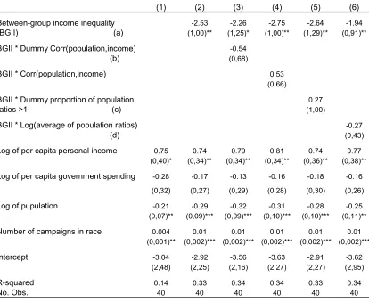
The estimation results are reported in table 3. As measure of between-group income inequality it is used the standard deviation of the log of the MSAs’ per capita income.15 The columns differ in the control variables included. Standard deviations are robustly estimated. In the line of some recent studies (e.g. Ansolabehere, et al., 2002), there is evidence that campaign contributions are not a form of policy-buying, but rather a form of political consumption. This conclusion comes from the fact that the government spending is not relevant in explaining campaign spending whereas personal income is. The income elasticity is quite near to that found in previous studies.

Concentrate now in the between-group inequality. Column 2 in table 3 presents the results when the campaign spending is controlled by this variable. As we expected, the sign of the respective parameter is negative, i.e. a higher between-group income inequality implies a lower level of conflict. Moreover, this parameter is significantly different from zero. This evidence supports the predictions of our theoretical model.

Since both the correlation between population and income and the percentage of population ratios equal or higher than one are low in some states, the sign of our relevant parameter might be the opposite for some states. Columns 3 through 6 in table 3 report some results that exploit explicitly the relationship between population and income. We do it by using the three measures mentioned above.

14 _{The only exception is Nevada, where this correlation is negative.}

15 _{The results are quite similar when we use alternative inequality measures as the variance of MSAs’ per}

Table 3

U.S. State Campaign Spending in House Race (Cycles 1991/92 to 1995/96)

Dep. Var.: Log of state per capita spending in House race. OLS estimation.

(1) (2) (3) (4) (5) (6)

Between-group income inequality -2.53 -2.26 -2.75 -2.64 -1.94

(BGII) (a) (1,00)** (1,25)* (1,00)** (1,29)** (0,91)**

BGII * Dummy Corr(population,income) -0.54

(b) (0,68)

BGII * Corr(population,income) 0.53

(0,66)

BGII * Dummy proportion of population 0.27

ratios >1 (c) (1,00)

BGII * Log(average of population ratios) -0.27

(d) (0,43)

Log of per capita personal income 0.75 0.74 0.79 0.81 0.74 0.77 (0,40)* (0,34)** (0,34)** (0,34)** (0,36)** (0,38)**

Log of per capita government spending -0.28 -0.17 -0.13 -0.16 -0.18 -0.16

(0,32) (0,27) (0,29) (0,28) (0,30) (0,26)

Log of pupulation -0.21 -0.29 -0.32 -0.31 -0.28 -0.25 (0,07)** (0,09)*** (0,09)*** (0,10)*** (0,10)*** (0,11)**

Number of campaigns in race 0.004 0.01 0.01 0.01 0.01 0.01 (0,001)** (0,002)*** (0,002)*** (0,002)*** (0,002)*** (0,002)***

Intercept -3.04 -2.92 -3.56 -3.63 -2.91 -3.62

(2,48) (2,25) (2,16) (2,27) (2,27) (2,95)

R-squared 0.14 0.33 0.34 0.34 0.33 0.34

No. Obs. 40 40 40 40 40 40

Standard deviations are robustly estimated. *** = Significant at the .01 level; ** = .05 level; and * =.1 level. (a) Between-group income inequality: Corresponds to the within state standard deviation of log of MSA per capita personal income; (b) Dummy Corr(population,income): 1 if the MSA correlation between population and per capita income is smaller that 0,23; (c) Dummy proportion of population ratios >1: 1 if the percentage of population ratios between richer and poorer cities higher that one is smaller that 50%; (d) Log(Average of population ratios): Correspond to the log of the average of population ratios between richer and poorer cities. The population ratios between richer and poorer cities correspond to all the possible population ratios between pair of MSA that have in the numerator the population of a richer city and in the denominator the population of a poorer one.

The second variable is the percentage of cases in which the population ratios are equal or higher than 1. Once more, we create dummy variables for different intervals of this percentage and introduce interaction between that and the between-group inequality. There is not any significant effect. Column 5 reports the regression with the best fit, where the dummy variable takes the value of one if the percentage is smaller than 50% and 0 otherwise.

Finally, we use the log of the average of population ratios. We introduce an interaction between this variable and the between-group inequality, which may allow us to obtain not only a different magnitude for the inequality effect in each state but also a different sign for those states where the average of the ratios is smaller than one. The parameter related to this interaction is negative, as we expect, but it is not significantly different from zero.

As our theoretical model predicts, the results for the political campaign spending case support the idea that the between-group income inequality affects the level of conflict in a society, and that, this effect depends on the relationship between group size and income. For this particular case, we have found that on average a higher between-city income inequality implies a lower level of campaign spending.

6.

Conclusions

This paper studies how the interaction among group-size, wealth, and its distribution affects both conflict intensity and group success probabilities in a society when there is a contest for either a pure public prize or a mix private-public prize. Different to the traditional studies on this topic, in this paper we assumed that conflict is due to differences in preferences for social outcomes that are not necessarily related to the individual wealth, and in particular is not generated by income inequality.

Using a contest model between interest groups that introduces explicitly the individual wealth, we find some interesting results. First, poorest people generally are not willing to engage in any conflict. Second, less inequality does not imply less conflict intensity. In fact, the “pure” effect that income redistribution has over the level of conflict is positive. Only under some especial conditions (when the poorer groups have a higher winning probability than the richer ones), income redistribution reduces the conflict intensity.