Performance predictability of divide and conquer skeletons

Performance Predictability of Divide and Conquer Skeletons

Fernando Saez Marcela Printista

LIDIC

Universidad Nacional de San Luis. Ej´ercito de los Andes 950, San Luis, Argentina. e-mail:f[email protected], [email protected]g

Abstract

Parallel divide and conquer computations, encompassing a wide variety of applications, can be modeled and encapsulated as a high level primitive called skeleton.

The paper deals with a skeleton designed for parallel divide and conquer algorithms that provide hyper-cubical communications among processes The paper also introduces an accurate timing model designed for prediction of proposed primitive. The timing analysis model presented here still characterizing the commu-nication time through architecture parameters but introduces a few novelties. The proposal is to introduce different kinds of components to the analytical model by associating a performance constant for each specific conceptual block of the skeleton. The trace files obtained from the execution of the resulting code using the skeleton are used by lineal regression techniques giving us, among other information, the values of the param-eters of those blocks. An extended example showing the relative accuracy of the proposed approach concludes the paper.

Keywords: Paralellism, Parallel Model, Skeleton, Timing Analysis, Divide and Conquer

1

INTRODUCTION

Traditionally, parallel programs are designed using low-level message passing libraries, such as PVM or MPI. Message passing provides the two key aspects of parallel programming: (1) synchronization of processes and (2) communications between processes. However, programmers still encountered difficulties because these interfaces force to deal with low-level details, and their functions are too complicated to use for a nonexpert parallel programmer.

Many attempts have been undertaken to hide parallelism behind some kind of abstraction in order to free the programmer from the burden of dealing with low level issues.

2

MOTIVATION

An alternative to the parallel programming is to provide a set of high-level abstractions which provides support for the mostly used parallel paradigms. A programming paradigm is a class of algorithms that solve different problems but have the same control structure. Programming paradigms usually encap-sulate information about useful data and communication patterns, and an interesting idea is to provide such abstractions in the form of programming templates or skeletons. In parallel context, the essence of this programming methodology is that all programs have a parallel component that implements a pattern or paradigm (provided by the skeletons) and a specific component of an application (in charge of the user). After the recognition of parallelizable parts and an identification of the appropriate algo-rithm, a lot of developing time is wasted on programming routines closely related to the paradigm and not the application itself. With the aid of a good set of efficiently programmed interaction routines and skeletons, the development time can be reduced significantly. The skeleton hides from the user the specific details of the implementation and allows the user to specify the computation in terms of an interface tailored to the paradigm.

To develop a specific application, the programmer/user chooses one or several skeletons, cus-tomizes them for the application and, finally, composes customized components together to obtain the executable target program. For example, we are familiar with concepts such as ”pipeline”, ”pro-cessors farms”, ”divide and conquer”, ”dynamic programming”, ”simulating annealing” and, more recently, those related with optimization problems. Before a new problem, we may try to formulate a solution in one of these well known styles. Since we already know how to implement the essential computational structure of each technique, it will only be necessary to introduce problem specific details to obtain a parallel version.

3

ABSTRACTION PRIMITIVE: DIVIDE AND CONQUER SKELETON

The Divide and Conquer approach (DC) finds the solution of a problemxby dividingxin

subprob-lems x 0 and

x

1. This procedure is applied recursively to solve a problem where subproblems are

smaller versions of the original problem. In this typical structure, the two subproblems can be done in parallel (Fig. 1). Infinite recursion is prevented using a predicatetrivial. If this predicate returns

TR UE, the functiononquer is applied to solve the problem directly without any further division.

At the ending of the procedure, the functionombineis used for merge the subsolutions in a general

solution.

1 procedure DC(p: Problem, r: Result) 2 begin

3 if trivial(p) then conquer(p, r); 4 else

5 begin

6 divide(p, p0, p1);

7 do in parallel (DC(p0,r0), DC(p1,r1) ); 9 combine(r, r0, r1);

10 end; 11 end;

Figure 1: ParallelD&C approach

From the experience obtained in the programming skeletal, especially in the design of different skeletons [7, 5], we have implemented a versatile parallelDivide and Conquerskeleton [6] .

The prototype for skeletonDC Call is as follows:

void DC_Call(typeDC Type, int Weight, mInteraction IM, TPF_trivial Itrivial, TPF_conquer Iconquer, TPF_divide Idivide, TPF_combine Icombine, TPF_secuencial Isecuencial,

TypeN *In,int SizeBufferIn, int SizeDataTypeIn, TypeN *Out, int SizeBufferOut,

int SizeDataTypeOut, MPI_Comm comm)

The parameters number in the call to the skeleton DC Call, may look a little complex, but this

long parameter list allows substantial flexibility, which will bring benefits in different domains. The first parameter (an enumerate type) specifies the type of algorithm to be used, which will depend of the specific problem to solve. In this work, we explore Hypercube Divide and Conquer, HDC.

This type provides a structure with hypercubical communications among processes. It generates, recursively, a binary tree of groups of processes whose leaves consist of only one process. The number of processes in each branch is halved at each level and its interactions within a level occur between pairs of processes which will have the same rank (in distinct groups) at the next level down. There are other types ofDC algorithms, such as Classical Divide and Conquer, Divide and

Con-quer with Embarrassing Divisibility and Divide and ConCon-quer with Trivial Combine Operation. In the first type of algorithm, the input is presented in only one processor. When the computation reaches the division phase, the processor will communicate the subproblems to the available processors and it will continue with its subproblem. In the Divide and Conquer with Embarrassing Divisibility type, the communication is not necessary. This structure is common in many algorithms whose data are totally distributed. Examples are the scalar product and the balanced matrix multiplication. In the third type, once the final point of recursion is reached, the leave processes will have the solution to the total problem in a distributed way. For example, mergesort has a trivial divide operation.

The body of the routinestrivial,sequential,divideandombineare described by functions and

they will need to be implemented by the user.

4

PERFORMANCE PREDICTABILITY

A computational model is an abstract computing tool used to reason about computation. Algorithm complexity depends on the computational model in which the algorithm is defined. Some models are necessarily elaborate and include a large number of parameters. There are other models of complexity likeLogP orBSP, characterizing the performance of distributed machines through a few architecture

parameters but they incur in a considerable loss of accuracy [3].

The advantage of using skeleton is the availability of a formal framework for reasoning about programs. In addition, cost measure can be associated with skeletons, thus enabling performance considerations. The timing analysis model presented here still characterizing the communication time through architecture parameters but introduces a few novelties.

The proposal is to introduce different kinds of components to the analytical model by associating a performance constant for each specific conceptual block of the skeleton.

The proposed parallel computational model considers a cluster made up by a set ofP processing

elements and memories connected through a network. The computation in the model involves three kinds of components:

Common pattern of paradigm: sequence of local operations needed to implement the paradigm.

User functions of paradigm: sequence of operations on local data needed to implement the

Communications: exchange of data among two or more processes in one or more processors.

Some of these components can be dropped in some type of skeleton, therefore, a skeleton model is characterized by the way it does each of the three previous components.

In conclusion, the model is characterized by the tuple:

( sk ; f 1 ;:::; f n

;g;l;P) (1)

The conceptual blocks f

i

will depend on the specific application and, in this case, they will be obtained by means of a description provided by the designer of the application.

Associated with these components there are cost functions. The function

skcorresponds to the

time invested in computation by the skeleton (implementation of paradigm), the function

Exis the

analytical communication model and it plays an important role in prediction of the execution time of parallel applications on parallel machine and functions

fi are associated to the cost of each specific

function involved in the particular skeleton (user functions). The costof a skeleton is given by:

SK ;P

=F( sk ; f1 ;:::; fn ; Ex ) (2)

The values of sk

; fiand

Extypically depend on the number of processors

P and on the problem

sizeSIZE.

The time

Ex predicts the time invested in communications. In addition to

P and SIZE, it

de-pends on the value of two determinants parameters to evaluate computational capacity of a parallel machine. In skeletons like Hypercube Divide and Conquer (HDC) where many sources are

contin-uously sending data to many processors, we use an average data full throughputg

ful l and a latency

l, both dependent onP. In this case the communication bottleneck is the transfer capacity of the

network.

In skeleton DC Call, Ex

(K;g (ful l ;P)

;l P

) represents the data exchange phase, and it can be

formuled by means of the following equation:

Ex

(K;g (ful l ;P)

;l P

)=t send

(K;g (ful l ;P)

;l P

)+t rev

(K;g (ful l ;P)

;l P ) wheret sendand t

revrespectively denote the time to send and receive a block containing

K

con-tiguous data units. Our communication model is linear, representanting the communication time by a linear function of the message size:

t send

(K;g (ful l ;P)

;l P

) = (l P

+Kg (ful l ;P)

)

t rev

(K;g (ful l ;P)

;l P

) = (l P

+Kg (ful l ;P)

)

The communication time can be summarized as follows:

Ex

(K;g (ful l ;P)

;l P

)=2((l P

+Kg (ful l ;P)

))

The parameters needed to design the model are not only architecture dependent (P;l;g)but also

it must be reflect skeletal characteristics ( sk,

f

i). The dependence of the architecture allowed in

5

PERFORMANCE PREDICTABILITY OF HYPERCUBE DIVIDE AND

CONQUER SKELETON

Next, we present and verify an accurate timing parallel model of computation developed to analyze and to predict performance ofHDCalgorithms using the skeletonDC Call.

In order to achieve an instance model of HDC, we need to describe the cost functions. As we

have previously seen, a divide and conquer problem needs to define five specific functions: trivial,

onquer, divide, ombine and sequential. We do not include costs associated with tasks trivial

andonquer since they do not make a significant contribution to execution time whenSIZE much

bigger thanP.

The parallel time of anHDCalgorithm with input sizeSIZEcan be formulated as a function of

five parameters:

HDC ;P

(SIZE)=F( HDC ; Div ; Comb ; Seq ; Ex ) (3)

The communication time of a cluster ofP processors can be described by machine-dependent

pa-rameters:g, the time needed to send one data word into the communication network, or to receive one

word, in the asymptotic situation of continuous message traffic andl, the latency or startup cost. They

are well known in parallel models area, and they are easy to obtain from any cluster. So, associated to the stage of communication between partners there is a cost function

Ex

(SIZE;g;l;P)which

gives us a time prediction invested for communications in terms of number of processors (P) in the

work group and the lengths of messages involved. In this case,

HDC is considered zero because

HDC is insignificant compared to other

compo-nents affecting the overall. Next, we need to find a different proportionality constant (cost) for each specific function.

The time HDC ;P

(SIZE)taken byP processors using the skeletonDC Call is recursively

de-fined by the formula:

HDC;P

(SIZE) = max i=1;:::;P

f Div;i

(SIZE)g+ max i=1;:::;P f HDC;P ( SIZE 2 )g+ max i=1;:::;P f Ex;i

(K0;g;l )g+ max i=1;:::;P

f Comb;i

(SIZE)g

HDC can be derived by successive substitution:

HDC;P

( SIZE

2

) = max

i=1;:::;P f Div;i ( SIZE 2

)g+ max i=1;:::;P f HDC;P ( SIZE 4 )g+ max i=1;:::;P

fEx;i(K1;g;l )g+ max i=1;:::;P f Comb;i ( SIZE 2 )g HDC;P ( SIZE 4

) = max

i=1;:::;P f Div;i ( SIZE 4

)g+ max i=1;:::;P f HDC;P ( SIZE 8 )g+ max i=1;:::;P f Ex;i (K 2

;g;l )g+ max i=1;:::;P f Comb;i ( SIZE 4 )g

And so on. When processors finish the recursion, the time is given by:

HDC;P

( SIZE

2 (logP) 1

) = max

i=1;:::;P f Div;i ( SIZE 2 (logP) 1

)g+ max i=1;:::;P f HDC;P ( SIZE 2 logP )g+ max i=1;:::;P f Ex;i (K (logP) 1

;g;l )g+ max i=1;:::;P

f Comb;i

( SIZE (logP) 1

AfterlogP division steps, the algorithm resolves each subproblem in a sequential form:

HDC;P

( SIZE

2 logP

)= max i=1;:::;P

f Seq;i

( SIZE

2 logP

)g

The cost of an algorithm is simply the sum of the costs of its components:

HDC;P(SIZE) =

(logP) 1 X

j=0 max i=1;:::;P

fDiv;i( SIZE

2 j

)g+ (logP) 1

X

j=0 max i=1;:::;P

f Comb;i

( SIZE

2 j

)g

+ (logP) 1

X

j=0 max i=1;:::;P

f Ex;i

(kj;g;l )g+ max i=1;:::;P

f Seq;i

( SIZE

2 logP

)g

5.1 Measuring Communication Performance

Different proposals can be used to determine

Ex. For example, it would be valid to take as

Exthe

empirical set of linear by pieces functions obtained from Abandahs [2] or Arruabarrenas [4] studies, where latency and bandwidth are considered depending on the communication pattern. On other hand, it would be valid to evaluate the effective latency and throughput of message transmissions using a classical round-trip test (also called a ping-pong test) between two machines. The ping-pong test measures the time needed for a message of a given length to go from one machine to the other and to come back immediately.

The timming model presented characterizing the communication time through architecture param-eters and message size. It assumes a linear by pieces behaviour in the message size of the functions in

Ex. However, this behaviour can be non-linear in the number

P of processors (i.e. broadcast usually

have a logarithmic factor inP).

To obtain the architecture parameters, we used micro-benchmarks [1]. they were run in a dedicated fashion, i.e. no other user programs or unnecessary system services were allowed to run during the benchmarking. We considered two micro-benchmarks to measure; (1) The worst casel(latency) and

(2) The worst caseg

ful l, measured for data full all-to-all collective communication (throughput). Each

one of them was calculated for two different methods; (1) Let the message size vary and (2) Let the number of messages vary.

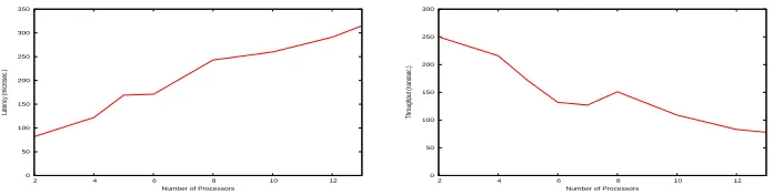
The Figure 2 shows the parameters for the clusterLIDIC. The cluster consisting of 14 networked

nodes, each one a Pentium IV of 3.2 GHz and 1 GB of Ram. The nodes are connected together by Ethernet segments and a Switch Linksys srw2024of 1GB. The base software on cluster include a

Debian etch SO, and MPICH 2 1.0.6. In both graphics, they-value corresponds to the time it takes

for a single integer (32-bit word) to be delivered. Note the latency increases much faster than the throughput decreases. Also note that the scale of the y-axes differ a factor1000. One may conclude

that latency becomes the most important factor when the number of processors grows.

Next sections exemplify the use of the model to predict the time spent by aHDCalgorithm.

6

CASE STUDY: CONNECTED COMPONENT

0 50 100 150 200 250 300 350

2 4 6 8 10 12

Latency (microsec.)

Number of Processors

0 50 100 150 200 250 300

2 4 6 8 10 12

Throughput (nanosec.)

Number of Processors

Figure 2:Latency and Throughput on Cluster LIDIC

2

1 3 4

5 6

7 8 9

Figure 3: Example of a graph

andjEj=M edges. The connected components ofGare the sets of nodes such that all nodes in each

set are mutually connected (reachable by some path), and no two nodes in different sets are connected. As a case of study we propose a parallel divide and conquer algorithm to identify subgraphs of the graph in which the nodes of the subgraph are connected.

We use a simple edges list to represent the graph. If G = (V;E) is a graph, its edges list is a

structure X

Mx2, where each edge e

i

= (u;v) 2 E, u < v, is stored in X[i℄, and X[i;0℄ = u y

X[i;1℄=v. The algorithm takes as input the edges list of a graphG(N nodes andM edges) stored

in a generic structureVetorInput. The procedure keeps for each node in the graph, all other nodes

which it has an edge to (the adjacency list of a node). The algorithm produces as output a vector

VetorOutput, where each element VetorOutput[j℄ for 1 j N will store the root of the

connected component forv j.

The following main program shows the connected components algorithm using the skeletonDC Call:

Algorithm ParallelConnectedComponent() initPar(&VectorInput,&VectorOutput,N,M);

DC_Call(HDC, 2, &trivial, &conquer, &divide, &combine, &secuencial, MPI_COMM_WORLD, &VectorInput, M, sizeof(edge), &VectorOutput, N, sizeof(int));

The first argument is used to specify the D&C type. In this case, it is a Hypercube Divide and

Conquer algorithm. The second parameter indicates the ramification factor. ForHDC,Weightmust

be equal to2(the number of activities generated in the division phase). The next five arguments are

used to introduce the specific code of application (user functions).

Here, we give a little example to show how the parallel algorithm works when using four proces-sors. Consider the graph as shown in the Figure 3, wherejEj=M =9andjVj=N =9.

The edges list<(1;2);(2;3);(1;3);(4;5);(5;6);(6;7);(4;7);(5;7);(8;9)>is stored in

Vector-Input.

The procedure divide divides the edges list in two of about n=2 edges each. Each of which is

then solved by applying the same approach recursively. Once we have reached a base case (trivial), a functionconqueris applied to find the roots of the connected components of its subedges list.

In the above example,VectorOutputassociated to processorP

iwould then look like:

P2:<1;2;3;4;4;4;7;8;9>

P3:<1;2;3;4;5;4;4;8;9>

P4:<1;2;3;4;5;6;5;8;8>

WhereVetorOutputassociatedP

icontains the roots of the connected components of its subedges

partition. For example, in the processorP

1, the node

1, 2and 3in the graphG belong to the same

subgraph with root in node1.

Then, the functioncombinecan just merge this sublist with its level partner to produce a new root vector of connected components. After the firstmerge, theVectorOutputswill be as follows:

P 1:

<1;1;1;4;4;4;7;8;9>

P 2:

<1;1;1;4;4;4;7;8;9>

P 3:

<1;2;3;4;4;4;4;8;8>

P4:<1;2;3;4;4;4;4;8;8>

After the lastmerge, theVectorOutputswill be as follows:

P 1:

<1;1;1;4;4;4;4;8;8>

P2:<1;1;1;4;4;4;4;8;8>

P3:<1;1;1;4;4;4;4;8;8>

P4:<1;1;1;4;4;4;4;8;8>

The list identifies the root of each connected component. It can be seen that the root of a compo-nent is the member node with lowest visitation index.

7

MEASURING OF D&C FUNCTIONS OF CONNECTED COMPONENT

To predict the time ofHDCalgorithms is necessary to estimate the execution time of each function

implemented by the user (divide,ombineandsequential) on the cluster.

The algorithm takes as input two parameters: the number of nodes (N) and edges (M). Each

parameter affects in some way to the specific function. In the functiondivide, the number of edges

of the graph plays a fundamental role to estimate the cost. On the other hand, the number of nodes determines the behavior for functionombine. The functionsequentialis affected by both variables.

Multivariate statistics refers to a group of inferential techniques that have been developed to handle situations where sets of variables are involved as predictors of performance. We make use of statistical analysis for determining model coefficients.

A model relating the experimental execution time of functiondivideto a set of independent

vari-ables is: T Div

=Div 0

+Div 1

M where1andM are the basis functions of the model andDiv iwill

be estimated by the parameter estimation algorithm. Linearleast-squares models (LSQ)estimate the coefficientsDiv

0 and Div

1to minimize the squared sum of errors between predicted and

experimen-tal values of functiondivide. The execution time model of functionombineis obtained in a similar

way:T Comb

=Comb 0

+Comb 1

N, whereComb 0and

Comb

1 are their unknown coefficients.

Each data in the trace file is used like input for regression techniques to find coefficients that achieve the best approximation to the real function.

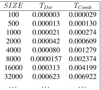
The function sequential has a cost of O(2N +M). To build an adjacency list, it requires N

Div Comb

100 0.000003 0.000029 500 0.000013 0.000130 1000 0.000021 0.000274 2000 0.000042 0.000609 4000 0.000080 0.001279 8000 0.0000157 0.002374 16000 0.000313 0.004199 32000 0.000623 0.006922

. . . .

Table 1: Trace file of experimental execution times of functionsdivideandombine

From our algorithm, DFS with adjacency list requires time proportional toO(N +M). The table

2 shows a sample of invested time for functionsequential. We can see it is linear in the size of the

structure. The values ofSeq 0,

Seq 1 and

Seq

2 will be obtained from regression techniques and they

conform the coefficients ofT S

eq =Seq 0

+Seq 1

N +Seq 2

M.

N M T

Seq

N M T

Seq

4000 4000 0.000960 16000 4000 0.001182 4000 8000 0.01804 16000 8000 0.002264 4000 16000 0.003624 16000 16000 0.004386 4000 32000 0.008119 16000 32000 0.009350 8000 4000 0.001065 32000 4000 0.001411 8000 8000 0.002029 32000 8000 0.002537 8000 16000 0.003962 32000 16000 0.004929 8000 32000 0.008445 32000 32000 0.010441

Table 2: Trace file of real execution times of functionsequential

The table 3 shows the estimated values for approximation functionsdivide,ombineandsequential.

In all cases, the coefficients of determination exceed95%.

division Div

0

Div 1

(R 2

)

1:94e 08

2:25e 06

99%

ombine Comb

0

Comb 1

(R 2

)

2:19e 07

2:32e 03

95%

sequential Seq 0

Seq 1

Seq 2

(R 2

)

0 1:35e

07

4:60e 07

98%

Table 3: Numerical value of coefficients

Results

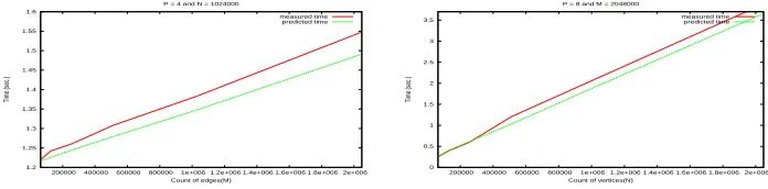
We performed initial experiments. The table 4 shows the execution time for several problem sizes using 8 processors.

To predict performance of some instances, the prediction model HDC ;P

(Size)was resolved

Par

8 1024000 512000 1.719770 8 1024000 1024000 1.844182 8 1024000 2048000 2.102299 8 2048000 512000 3.002905 8 2048000 1024000 3,128890 8 2048000 2048000 3.504908

Table 4: Times to find connected component using parallel algorithm

1.2 1.25 1.3 1.35 1.4 1.45 1.5 1.55 1.6

200000 400000 600000 800000 1e+006 1.2e+006 1.4e+006 1.6e+006 1.8e+006 2e+006

Time (sec.)

Count of edges(M) P = 4 and N = 1024000

measured time predicted time

0 0.5 1 1.5 2 2.5 3 3.5

200000 400000 600000 800000 1e+006 1.2e+006 1.4e+006 1.6e+006 1.8e+006 2e+006

Time (sec.)

Count of vertices(N) P = 8 and M = 2048000

measured time predicted time

Figure 4: Measured Time vs Predicted Time for different configurations.

execution time to find connected components for a graphG = (V;E) with jVj = N = 1024K y

jEj=M =2048K using8processors.

To estimate the time spent in communication, we instantiatet

Exwith the number of words

(32-bit) to communicate by each recursion level and the architecture parameters (landg). For this

prob-lem, each algorithm recursion level always communicates the whole root’s vector, this is1024K of

32-bits words.

2 X

j=0 max i=1;:::;8

f Ex;i

(1024K;1:5110 7

;2:4310 4

)g = 32(0:000243+1024K 1:5110 7

)

= 32(0:000243+0:154624)=0:929202

The predicted time to solve the connected components of a graphGis the sum of the time invested

for each component function:

HDC ;8

(1024K;2048K)=1:916492

In this particular prediction the error was 8;83%. (Predicted = 1.916492 versus Observed=

2.102299, see table 4). Errors are basically due to the lack of accuracy for the communication com-ponent.

The figure 4 shows a comparison between predicted time and the traces obtained for several con-figurations. The results were very near to the expectable behaviour.

8

CONCLUSIONS AND FUTURE WORK

In this paper, we first described the skeleton DC Call. It provides high-level abstraction for

synchronization. The results obtained using the skeleton described in this paper prove it to be suit-able to handle the class of problems parallel divide and conquer. The application programmers benefit from proposed skeleton, which hides much of the complexity of managing parallel divide and conquer algorithms. We believe that preserving the semantics of the sequential divide and conquer program is a key point to achieve the objective to alleviating the difficulties in the development of parallel applications.

Besides this, the paper also presents and verifies an accurate timing model to predict the perfor-mance of the proposed primitive on a clusters of processors. The parameters needed to design the model are not only architecture dependent(P;l;g)but also it must be reflect skeletal characteristics.

The dependence of the architecture allowed in the cost functions is in the coefficients defining each particular function of the skeleton DC Call. Thus, once the analysis for a given architecture has

been completed, the predictions for a new architecture can be obtained replacing in the formulas the function coefficients. We used statistical analysis for determining analytical model coefficients. The multivariate techniques described here are particularly applicable because of the large number of sam-ples the system allows to obtain. In this way, the programmers are provided with a high level primitive whose different implementations have a well-understood behaviour and predictable efficiency.

Future work should concentrate in describing other abstraction primitives and to extend the skele-ton’s portability to support both shared and distributed memory architectures.

ACKNOWLEDGMENTS

We wish to thank the Universidad Nacional de San Luis, the ANPCYT and the CONICET from which we receive continuous support.

REFERENCES

[1] Mpiedupack 1.0. available at http://www.math.uu.nl/people/bisseling/edupack/mpiedupack1.0.tar.

[2] Davidson E.S. Abandah, G.A. Modeling the Communication Performance of the IBM SP2. Proc. 10th IPPS., 1996.

[3] Printista A.M. Modelos de Predicci’on en Computaci’on Paralela. Thesis of Magister submitted to the Universidad Nacional del Sur., 2001.

[4] Arruabarrena A. Beivide R. Gregorio J.A. Arruabarrena, J.M. Assesing the Performance of the

New IBM-SP2 Communication Subsystem. IEEE Parallel and Distributed Technology. pp 12-22.,

1996.

[5] C. Rodriguez Len F. Piccoli, M. Printista.Dynamic Hypercubic Parallel Computations. Proceed-ing (466) Parallel and Distributed ComputProceed-ing and Systems, 2005.

[6] M. Printista F.D. Saez. Programacin Paralela Esqueletal. XIII Congreso Argentino de Ciencias de la Computacin, Corrientes and Resistencia, Argentina, October 2007.