ON THE USE OF THE MP3 FORMAT AND M SEQUENCES APPLIED TO ACOUSTIC MEASUREMENT

ON THE USE OF THE MP3 FORMAT AND M SEQUENCES APPLIED TO

ACOUSTIC MEASUREMENT

PACS REFERENCE: 43.60.Bf

Paulo, J. V. C. Preto1; Martins, C. R.1; Coelho, J. L. Bento2

1

Escola Náutica Infante D. Henrique Av. Eng. Bonneville Franco

Paço D'Arcos - 2780 Oeiras Portugal

email: joelpaulo@enautica.pt email: carlosmartins@enautica.pt

2

CAPS - Instituto Superior Técnico Av. Rovisco Pais, 1049-001

Lisboa Portugal

ABSTRACT

Acoustical measurement systems based on computers are very popular, nowadays.

In some applications, such as environmental noise, industrial noise or in sportive/cultural events, large data acquisition times are required. The captured data is then stored and post-processed at the laboratory.

In such cases, large storage platforms must be accessible in situ to accommodate all the information.

This paper focuses on the use of the MPEG 1/2 Layer 3 (MP3) in acoustics in order to reduce importance of the computer’s storage capabilities.

Various examples are presented by comparing the performance of the classic MLS technique with and without audio compression using the MPEG3 format. Advantages and disadvantages are discussed.

1. INTRODUCTION

The goal of this work is to compare the performance of the Impulse Response measurements using the MLS technique with and without the MP3 data compressed audio format.

1.1 Brief Introduction to MP3 Format

Algorithm description

1.1.1 Filterbank

The filterbank used in MPEG-1 Layer-3 belongs to the class of hybrid filterbanks. lt is built by cascading two different kinds of filterbanks: Firstly, the polyphase filterbank (as used in Layer-1 and Layer-2) and then an additional Modified Discrete Cosine Transform (MDCT). The polyphase filterbank has the purpose of making Layer-3 more similar to Layer-1 and Layer-2. The subdivision of each polyphase frequency band into 18 finer sub-bands increases the potential for redundancy removal, leading to better coding efficiency for tonal signals.

Another positive result of a better frequency resolution is the fact that the error signal can be controlled to allow a finer tracking of the masking threshold. The filter bank can be switched to a lower frequency resolution in order to avoid pre-echoes.

1.1.2 Perceptual model

The perceptual model either uses a separate filterbank or combines the calculation of energy values (for the masking calculations) and the main filterbank. The output of the perceptual model consists of values for the masking threshold or allowed noise for each coder partition. In Layer-3, these coder partitions are roughly equivalent to the critical bands of human hearing. lf the quantization noise can be kept below the masking threshold for each coder partition, then the compression result should be indistinguishable from the original signal.

1.1.3 Quantization and coding

A system of two nested iteration loops is the common solution for quantization and coding in a Layer-3 encoder. Quantization is done via a power-law quantizer. In this way, larger values are automatically coded with less accuracy and some noise shaping is already built into the quantization process.

The quantized values are coded by Huffman coding. To adapt the coding process to different local statistics of the music signals the optimum Huffman table is selected from a number of choices. The Huffman coding works on pairs and, only in the case of very small numbers to be coded, quadruples. To get even better adaptation to signal statistics, different Huffman code tables can be selected for different parts of the spectrum.

Since Huffman coding is basically a variable code length method and noise shaping has to be done to keep the quantization noise below the masking threshold, a global gain value (determining the quantization step size) and scale factors (determining noise shaping factors for each scale factor band) are applied before the actual quantization.

The process to find the optimum gain and scale factors for a given block, bit-rate and output from the perceptual model is usually done by two nested iteration loops in an analysis-by-synthesis way:

• Inner iteration loop (rate loop)

The Huffman code tables assign shorter code words to (more frequent) smaller quantized values. lf the number of bits resulting from the coding operation exceeds the number of bits available to code a given block of data, this can be corrected by adjusting the global gain to result in a larger quantization step size, leading to smaller quantized values. This operation is repeated with different quantization step sizes until the resulting bit demand for Huffman coding is small enough. The loop is called rate loop because it modifies the overall coder rate until it is small enough.

• Outer iteration loop (noise control loop)

supplied by the perceptual model, the scale factor for this band is adjusted to reduce the quantization noise.

Since achieving a smaller quantization noise requires a larger number of quantization steps and thus a higher bit-rate, the rate adjustment loop bas to be repeated every time new scale factors are used. In other words, the rate loop is nested within the noise control loop. The outer (noise control) loop is executed until the actual noise (computed from the difference of the original spectral values minus the quantized spectral values) is below the masking threshold for every scale factor band (i.e. critical band).

Figure. 1. Block diagram of an MPEG – 1,2 Layer-3 encoder.

1.2 Brief Theory of M Sequences (MLS)

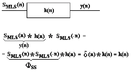
M Sequences are a special kind of correlation signals. The sequences are periodic binary (+1 and -1) pseudo-random signals. The auto-correlation function of these sequences result in a dirac impulse (excluding a very low DC value). In this sense, assuming a linear and time invariant system, the room impulse response is evaluated with the cross-correlation between the MLS and the signal at the reception point as it is shown in Figure 2,

Figure 2. Scheme of the impulse response calculation in a Linear Time Invariant System using the MLS technique.

the shift registers used for its generation. Each peak (dirac impulse) contains the same energy of the total length of the MLS.

Care must be taken in choosing the sequence length to avoid time aliasing [2]. This can be achieved by using a sequence duration (L / fs) corresponding to a value higher than the reverberation time of that room [3].

The cross-correlation is calculated by using the Fast Hadamard Transform - FHT [4, 5].

Figure 3 illustrates the MLS technique for the measurement of the room impulse response.

Figure 3. Minimal configuration for the impulse response measuring using the MLS technique.

In order to guarantee reliable results, it is very important to synchronize the input and the output signals. Furthermore, for adequate equalization purposes of the whole chain it is convenient to have proper knowledge of the frequency response of every piece of the measuring equipment [6].

2. METHOD

The work was conducted by comparing the original system Impulse Response with Impulse Response calculated by means of MLS technique with and without data compression (MP3). To evaluate the measure degradation the Quadratic Impulse Response Error, Quadratic Amplitude Impulse Response RT60 Error and RT60 Energy Error was investigated in octave bands.

The block diagram used in this analysis is depicted in Figure 4.

The impulse response was synthesized by using the mathematical expression depicted below, which nearly represents the exponential falling down of the acoustic energy inside a closed room.

h n

[ ]

=

e

*W[n]

fs – Sampling Frequency RT60 – Reverberation Time

W [n] – normally distributed random variable with zero mean and unity variance

The signals used in the simulations were compressed at different bit rates to evaluate the degradation in the acoustic tests results.

3. SIMULATION TESTS

The signals used in the simulations were compressed to 48, 80, 128, 192 and 320 bits/s which corresponds to a compression ratio of 14:1, 8:1, 5:1, 3:1 and 2:1 (mono signals) respectively.

The synthesised system Impulse Response used in tests corresponds to a RT60 of about 0.26s that simulates a small acoustical treated home studio.

To avoid time aliasing, an MLS of order 15 was used at a sample rate of fs = 44.1 kHz, which corresponds to a period of about 0,7 s.

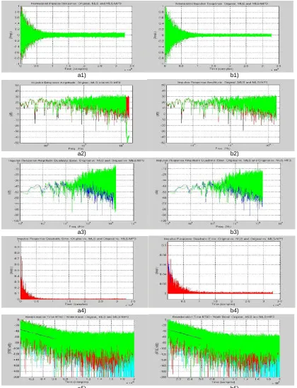
Results of the tests are depicted in figure 5 for two different bit rates.

The Impulse Response results show a considerable degradation. Notice the background noise of the Impulse Response and bandwidth reduction for 80 bits/s. To quantify these results the RT60 Error and the RT60 Energy Error were evaluated.

a1) b1)

a2) b2)

a3) b3)

a4) b4)

a5) b5)

Figure 5. Differences in behaviour between impulse responses calculated with and without compressed MP3 for 8 0 bits/s (sub-figures a1-5)) and 128 bits/s (sub-figures a1-5)). MP3 results

are the green curves except for the sub-figures a4) and b4) that are red curves. a1) and b1) Impulse Response. a2) and b2) Impulse Response Amplitude. a3) and b3) Impulse Response

Amplitude Quadratic Error. a4) and b4) Impulse Response Quadratic Error. a5) and b5) RT60.

a1) b1)

a2) b2)

a3) b3)

a4) b4)

a5) b5)

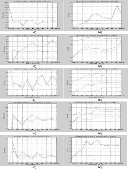
Figure 6. RT60 Error and the RT60 Energy Error - Errors of RT60_MLS with and without data compression. The errors are related to the original RT60. Indexes 1 to 5 correspond to the different bit rates analysed (1 – 48, 2 – 80, 3 – 128, 4 –192, 5 – 320 bits/s). The RT60 Error and

The results in figure 5 show that both RT60 and RT60 Energy errors decrease with the increase on the bit rate, as expected. For bit rates higher or equal to 128 bits/s, the RT60 Error is below 25 ms and the RT60 Energy Error is below 0.6 dB. For these bit rates admissible results can be achieved.

Note that the simulation results are invalid for the 31.5 Hz frequency band.

4. CONCLUSIONS

The MP3 data compression algorithm applied to the standard MLS technique was investigated to found some guidelines to its applicability in acoustics.

It was experimentally demonstrated that for bit rates higher or equal to 128 bits/s (that corresponds to a minimum compression ratio of 8:1 for mono signals) the results concerning to RT60 Error and RT60 Energy Error were satisfactory in most acoustical tests.

The averaging procedure is used to improve the Signal to Noise Ratio at the receiver point of the system. However, it is not compatible with data compression inherent to its perceptual model characteristics (psychoacoustic model). Therefore, the averaging procedure must be used before the data compression stage.

5. REFERENCES

[1] Brandenburg, K., "MP3 and AAC Explained", Audio Eng. Soc., 17th International Conference on High Quality Audio Coding.

[2] Rife, D. D., Vanderkooy, J., "Transfer-Function Measurement with Maximum-Length Sequences", J. Audio Eng. Soc., Vol. 37, No. 6 (1989)

[3] Vorlander, Michael, Mommertz, E., "Guidelines for the Application of the MLS Technique in Buildings Acoustics and in Outdoor Measurements", Inter-Noise 1997, Budapest - Hungary, August 25-27 (1997)

[4] Borish, J, Angell, James B., "An Efficient Algorithm for Measuring the Impulse Response Using Pseudorandom Noise", J. Audio Eng. Soc., Vol. 31, No. 7 (1983)

[5] Vorlander, Michael, "Aplications of Maximum Length Sequences in Acoustics", I Simpósio Brasileiro de Metrologia em Acústica e Vibrações. Petrópolis, RJ, Brasil, December 04-06, (1996)