Evaluating the transport in small-world and scale-free networks

(1)

Evaluating the transport in small-world and scale-free networks

R. Juárez-López

a,b

, B. Obregón-Quintana

a,c

, R. Hernández-Pérez

d

, I. Reyes-Ramírez

a

,

L. Guzmán-Vargas

a,⇑

a

Unidad Profesional Interdisciplinaria en Ingeniería y Tecnologías Avanzadas, Instituto Politécnico Nacional, Av. IPN No. 2580, L. Ticomán, México D.F. 07340, Mexico

b

Petróleos Mexicanos, Av. Prol. de Juárez, Comalcalco, Tabasco 86388, Mexico

c_{Facultad de Ciencias, Universidad Nacional Autónoma de México, Ciudad Universitaria, Mexico} d

SATMEX, Av. de las Telecomunicaciones S/N, CONTEL Edif. SGA-II, México, D.F. 09310, Mexico

a r t i c l e

i n f o

Article history: Received 14 March 2014 Accepted 10 September 2014 Available online 8 October 2014

a b s t r a c t

We present a study of some properties of transport in small-world and scale-free networks. Particularly, we compare two types of transport: subject to friction (electrical case) and in the absence of friction (maximum flow). We found that in clustered networks based on the Watts–Strogatz (WS) model, for both transport types the small-world configurations exhibit the best trade-off between local and global levels. For non-clustered WS networks the local transport is independent of the rewiring parameter, while the transport improves globally. Moreover, we analyzed both transport types in scale-free networks considering tendencies in the assortative or disassortative mixing of nodes. We construct the distribution of the conductanceG and flowF to evaluate the effects of the assortative (disassortative) mixing, finding that for scale-free networks, as we introduce different levels of the degree–degree correlations, the power-law decay in the conductances is altered, while for the flow, the power-law tail remains unchanged. In addition, we analyze the effect on the conductance and the flow of the minimum degree and the shortest path between the source and destination nodes, finding notable differences between these two types of transport.

1. Introduction

In recent years, researchers from different disciplines have shown an increasing interest in the study of complex networks [1,2,4,3]. In particular, several approaches to classify and characterize complex networks have been proposed, which aim to help in the understanding of the networks operation and organization under different con-ditions[5,6], and very recently researchers have addressed the multiplex character of real-world systems[7]. As it is well known, a network is comprised of a set of nodes or vertices, and the set of links or edges that interconnect

the nodes. The links can have a given direction and are known as directed; and in some cases they represent also a certain intensity in the connection which leads to net-works with weighted links. The degree of a node is deﬁned as the number of links that fall on it, when the links are not directed. However, in a directed network, the degree can be either interior (links coming into the node) or exterior (links coming out of the node). Moreover, the degree distri-butionPðkÞ, where kis the degree, allows describing the network connectivity, i.e., this distribution is obtained from plotting the frequencies against the degree, and char-acterizes the network; thus, the structure ofPðkÞprovides information on how the links are distributed [8,9]. For instance, it is known that random networks possess a char-acteristic connectivity scale[4], meaning that most of the

⇑ Corresponding author.

E-mail address:lguzmanv@ipn.mx(L. Guzmán-Vargas).

Contents lists available atScienceDirect

Chaos, Solitons & Fractals

Nonlinear Science, and Nonequilibrium and Complex Phenomena

(2)

nodes have an average number of links, that is described by a Poisson-like distribution. In many cases, real networks exhibit the small-world property, that is, the average path length is small and the clustering coefficient (local struc-ture) is high [10]. A representative small-world model was proposed by Watts and Strogatz[10], which interpo-lates between a regular clustered network and a random graph; for intermediate configurations the small-world feature is observed. Moreover, there are networks where the distribution has no characteristic scale so they are called scale-free networks for which a significant number of nodes coexist with few links and few highly connected nodes known as hubs. For these networks, the degree dis-tribution is given by a power law:PðkÞ kk

[9]. Recent studies on the transport properties in complex networks have reported that scale-free networks display better transport conditions than random networks, due to the presence of hubs[11,12]. Transport in non regular media, such as complex networks, provides an approach to the exploration of transport in many real conditions from elec-trical networks to the Internet[13–17]. Transport within a network consists of sending an entity from a specific node called the origin or source to another node called destina-tion or sink. This problem can be stated as a flow problem to find the paths from source to destination for which it is possible to send as much flow as possible while satisfying capacity constraints on the links and flow conservation at the intermediate nodes [18,19]. Moreover, transport in many real situations involves the presence of friction. These cases can be modeled using analogies with electrical systems: a positive potential is assigned to the origin node while a zero potential is assigned to the destination node, and the links are considered as resistors. Based on the law of conservation of electrical charge, it is possible to estimate the current flow from the origin to the destination. On the other hand, a complex network can be classified according to the bias or the degree–degree correlations, i.e., if there is a bias in the connectivity between nodes with high or low degree, then the network has assortative or disassortative mixing[20]. Here, we are interested in evaluating the transport properties in small-world networks and the effect of assortative (disassorta-tive) mixing on the transport in scale-free networks. Particularly, we focus on comparing the transport (with and without friction) in clustered and declustered small-world networks, by calculating the average conductance and the average flow on local and global scales; we find that for clustered networks and for both transport types, the best trade-off between local and global levels is observed for configurations with small-world topology, while for declustered networks, the transport improves globally and it is independent of the rewiring parameter. Besides, we also compare the effect of degree–degree correlations on the conductance and flow distributions in scale-free networks for three specific configurations. We observe a significant difference between the distributions for the three levels of assortative mixing. Our quantitative analysis also permits to test the effect on the conductance and the flow of the minimum degree and the shortest path between the source and destination nodes, finding notable differences between these two types of transport. The

paper is organized as follows: In Section2, a brief descrip-tion of small-world and scale-free network models is given. Next, Section3describes the way the degree–degree correlations are introduced. The results and discussion are given in Section4. Finally, in Section5some conclusions are presented.

2. Small-world and scale-free networks

Regular networks are the simplest model to describe the relationship between nodes since all nodes have the same degree; however, the model is not always appropri-ate to study real networks. An important model that inter-polates between a regular and a random network is the Watts–Strogatz model (WS) [10]: starting with Nnodes arranged in a ring with links to itsknext–nearest neigh-bors (a k-regular network), small-world conﬁgurations can be created through a rewiring process that with some probabilitypreassigns links (whenpis large enough, this rewiring process leads to a random network), creating shortcuts between distant sections of the ring. Thus, for

p¼0 we have the case of a clustered WS network whereas for intermediate values ofp, it is observed a high average clustering coefficient and short average path length, the main feature of the small-world network. A declustered WS model was proposed by Vragovic´ et al.[21]and con-sists in starting with a regular ring with next–nearest neighbor connections and adding links from each site to only its nth neighbors [21]. In this way, the initial configuration has zero clustering coefficient. In our study, we consider that shortcuts are created with a random rewiring process as in the ordinary WS model. We notice that in the declustered model proposed in [21], the rewiring procedure considers only the more distant neighbors of a given site, while nearest-neighbor links are kept unchanged. In our case, we consider clustered and declustered WS networks with the same size and equal number of initial edges.

Moreover in many real systems the description of the connectivities is given by a power-law/scale-free distribu-tion. An illustrative model to generate a scale-free network is that of Barabási–Albert where starting from a set of nodes with certain links, new nodes join according to the so-called preferential attachment process: nodes with more links are more likely to link new nodes [9]. The emerging network has a degree distribution of the power-law typePðkÞ kk

where the exponent,k, depends on the type of network under consideration[1]. A more appropriate model to generate scale-free networks with a random mixing and a deﬁned exponent, consists of using the Molloy–Reed algorithm on a set of Nnodes [22]: in which,ki copies for each nodeiare generated, where the probability of having a degree equal to ki satisﬁes

PðkiÞ kik. These copies of nodes are randomly linked, without repeating links and avoiding self-loops.

3. Degree–degree correlations

(3)

high-degree nodes. Such networks are said to display assortative mixing[20,23]. In contrast, when high-degree nodes tend to connect with low-degree nodes, it is said that the network has disassortative mixing. Several param-eters and quantities have been proposed to estimate the tendencies in assortative mixing. In 2002, Newman pro-posed ther-parameter deﬁned as the Pearson correlation coefﬁcient of degree between pairs of connected nodes, which is observed to lie within the interval 16_r6₁

[20]. For r>0, the network displays assortative mixing patterns, while forr<0, it exhibits disassortative mixing tendencies. Alternatively, other authors have proposed the measure knn¼Pk0kPðk0jkÞ, where Pðk0jkÞ is the

conditional probability that an arc coming out of a node of degreek points to a node of degreek0, for estimating the presence of correlations in a network[23]. Whenknn is an increasing (decreasing) function ofk, the network shows assortative (disassortative) mixing. Moreover, Doyle et al. proposed the quantitySto capture the tendencies in assortative mixing in a very direct way [24]; deﬁned as

S¼Pi;jkjki, where the sum operates over all pairs of nodes that are linked. Thus a high value ofSdenotes that high degree nodes are linked to each other and a low value indi-cates that high degree nodes are connected with low degree nodes. For the present study, we generate scale-free networks with exponent k¼2:5 using the Molloy–Reed method described above[22]. We use the criterion pro-posed by Doyle et al.[24]to generate three conﬁgurations: (i) assortativeSmax(ii) disassortativeSmin and (iii) neutral

Srand, as follows: ﬁrst, the nodes are sorted from highest to lowest degree. Then, to generateSmaxwe start from the node with the highest degree and subsequently create links to nodes in descending order until the degree is exhausted. In contrast to generateSmin, we start from the node with highest degree and links to nodes are created according to the ascending order. Finally, to generate

Srand, the nodes are randomly paired according to the degree of each node. In all cases, the repetition of links and the network disconnectedness shall be avoided.

4. Electric transport and max-ﬂow

To study some transport properties we calculated the conductanceGand maximum-ﬂowFbetween two nodes

AandBin both clustered/declustered Watts–Strogatz and scale-free networks, with different assortative mixing. The Kirchhoff’s laws are used to obtain G, imposing a potentialVA¼1 to the source node while the destination node is ﬁxed to zero potentialVB¼0. We also assume that all arcs have unitary resistance. We solve the system of lin-ear equations to determine the value of the potentialViin all nodes of the network. To estimate the total current enteringAand leavingB, the currents fromAto the nearest neighbors are added up, ﬁnding that the total current is numerically equal to the conductanceG[11].

For the case of frictionless transport, we use linear pro-gramming techniques[18]to calculate the maximum sta-tic flow (stable flow state) between nodesAandB; while the flow conservation law is used for intermediate nodes

[25]. Moreover, the capacity of the edges shall not be exceeded. In particular, in the present work the edges have

unitary capacity and the flow sent through any path is an integer amount of flow, and therefore, the flow is deter-mined by the number of edge-disjoint paths (paths that do not share any edges) from the sourceAto the destina-tionB[12].

In our analysis we calculate the global conductance (G) and maximum global ﬂow (F) as the average between all pairs of nodes, that is,

Gg¼

1

NðN1Þ

X

i–j

Gij ð1Þ

and

Fg¼

1

NðN1Þ

X

i–j

Fij: ð2Þ

We also compute both quantities locally, considering only the neighborhood of the nodei; Di, i.e., over all pairs of neighboring nodes of the node in question, including itself, and then averaging over all nodes in the network,

Gl¼

1

N

X

i

1

kiðkiþ1Þ X

s–t2Di

Gst ð3Þ

and

Fl¼

1

N

X

i

1

kiðkiþ1Þ X

s–t2Di

Fst; ð4Þ

wherekirepresents the degree of nodei.

4.1. Results for Watts–Strogatz networks

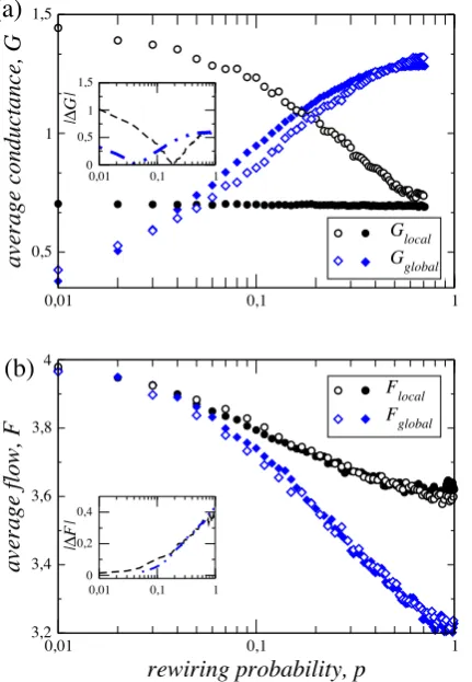
Fig. 1a shows the results of the network transport based

on the clustered and declustered WS model. In our simula-tions we considerN¼512 nodes, the number of neighbors

k¼4 for clustered networks, andk¼4 andn¼3 for the declustered model. For the electrical case and clustered WS model (Fig. 1a), the values for local and global average conductance are very different for regular settings (low

p), observing thatGl>Gg, which indicates that the trans-port is higher locally. By increasing the probability p; Gg increases whileGldecreases, revealing that the appearance of shortcuts allows the transport to increase globally while is locally low. In addition, for random networks (high val-ues ofp), it is observed thatGl<Gg. It is noteworthy that for conﬁgurations that are neither regular nor completely random, bothGlandGghave high values and, the absolute differencejDGj ¼ jGlGgjhas a minimum aroundp0:2 (see inset ofFig. 1a). From this we can conclude that trans-port within initial clustered networks with small-world topology is good both globally and locally. Moreover, for the declustered networks, the global conductance exhibit an increasing trend as the rewiring probability increases, whereas, the local conductance remains almost constant for different values of p, indicating that the presence of shortcuts improves the transport on global scale but not locally. When observing the absolute difference,

(4)

and declustered WS models displays that both local and global medium ﬂows decrease with the rewiring

probabil-ityp(Fig. 1b), such that the overall ﬂow decreases faster

while the local ﬂow reaches a higher value. In contrast to the electrical case and for clustered networks, the absolute differencejDFj ¼ jFlFgjshows an increasing behavior asp increases (see inset ofFig. 1b), indicating that both quanti-ties are quite similar at lowp(regular network), whereas for random conﬁgurations (p1) they exhibit a different average value withFl>Fg.

4.2. Results for scale-free networks

Given a scale-free network with degree distribution sat-isfying,PðkÞ kk, we manipulate the assortative mixing

introducing tendencies to generate networks matching the different cases Smax; Smin and Srand (see Fig. 2 for representative cases); and we proceed with computing bothGandFfor various conﬁgurations. In order to study the transport behavior, we compute the cumulative

(a)

(b)

Fig. 1.(a) Simulation results for the average global (Gg) and local (Gl)

conductance for different values of the rewiring probabilityp in the clustered (declustered) Watts–Strogatz model. For initial clustered WS networks, Gg (open diamonds) and Gl (open circles) follow opposite

trends for increasing p, and they intersect at p0:2 (see inset), suggesting that for a small-world conﬁguration both conductances reach intermediate values and the best trade-off between local and global levels. For initial non-clustered conﬁgurations, Gg (closed diamonds)

increases aspincreases, whileGl(closed circles) remains constant. The

inset shows the absolute differencejDGj ¼ jGlGgjfor both clustered

(dash line) and declustered (dash-dotted line) models. (b) Results for the maximum-flow vs.p. For clustered and declustered WS models, both the local and global flow decrease for increasing p, with the local flow decaying faster, suggesting that for random networks the capacity for frictionless flow is higher locally (the inset shows the absolute difference between the two flows). The results shown in (a) and (b) are average values obtained in 10 independent realizations.

(a)

(b)

(c)

Fig. 2.Representative cases of scale-free networks with different levels of assortative mixing: (a)Smin, (b)Srandand (c)Smax. For theSminconﬁguration

the nodes with high degree connect with low degree nodes, leading to ‘‘bottlenecks’’ in the communication with distant nodes. ForSmax, high

degree nodes connect between them, increasing the number of alternate paths to communicate two given nodes; whereas, forSrand, the

(5)

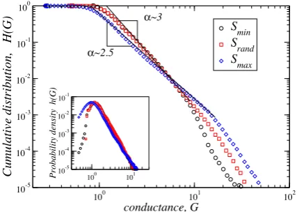
distribution functions (CDF)HðG>gÞandHðF>fÞwhich measure the probability of having conductances (or flow) greater than a given value.Fig. 3 presents the results for a scale-free network (k¼2:5) with different levels of assortative mixing. Note that for theSrandcase, the CDF in the first decade, 1<G<10, is well fitted by a power-law of the formHðGÞ Ga, with

a

¼2k2 [11,12]. As can be seen, difference in the distributions for large conduc-tances emerge when tendencies in the assortative mixing are introduced. For theSmax case, it is observed that the probability of having large values of the conductance (G>10) is greater than for the random case; while in the intermediate conductances range (1<G<10), the proba-bility for the random case is higher, indicating that the increase in the probability for large conductances is penal-ized with a decreasing of probability for low values ofG. However, a higher probability for large conductances rep-resents a higher transport capacity for networks with the

Smaxconﬁguration. In contrast, for theSmincase, the proba-bility of intermediate conductances (1<G<10), is very close to the random case, while the probability for large conductance (G>10) is smaller than Srand and Smax. For very small conductances range (G<1),Smaxshows a higher probability than the other two conﬁgurations (see inset of

Fig. 2). Therefore, we can conclude that the transport

capacity is affected by tendencies in the assortative mixing, being the random case the one with the best balance, despite the fact that the probabilities of the networks with

Smaxhave a higher probability for large conductances. To further explore the effects on transport of the assorta-tive mixing, we use the backbone picture proposed by López et al. [11], that is, we assume that the conductance,

G, between node A and B, can be expressed as 1=G¼1=GAþ1=GBþ1=GTB, whereGA(GB) andGTBrepresent the conductance of the neighborhood of nodeA(B), and the transport backbone, respectively. Following López et al., and assuming thatGA¼ckAandGB¼ckB, withca constant,

kA;kBthe degree of nodesAandB, respectively, we obtain

1=G¼ ðkAþkBÞ=ðckAkBÞ þ1=GTB. In order to estimate the effect of the assortative mixing over the transport backbone, for simplicity, we consider the symmetric casekA¼kB, and thus G¼ckA=ð2þckA=GTBÞ. Next, we consider ﬁrst-order approximation of the term ckA=GTB in the binomial ½2þckA=GTB1, leading toGckA½1=2ckA=ð

ffiffiffi 2

p

GTBÞ. To test the prediction of this approximation, we plotGvs.kA (Fig. 4) for the symmetric case (kA¼kB) in our simulation data. We identify two regimes, for small values, kA14, the quadratic term seems to be relevant, while for

kA>14, the linear behavior is quite dominant. For the quadratic regime, both conductances forSminandSrandshow the qualitative behavior predicted by the ﬁrst-order approximation, revealing that the backbone’s conductance inﬂuences the global electric transport. Surprisingly, for

Smax, the conductance is smaller than the other two conﬁgurations, which indicates that for low degree

100 101 102

conductance, G

10-5 10-4 10-3 10-2 10-1 100

Cumulative distribution, H(G)

S

min

S

_rand

S

max

100 101 10-5

10-4 10-3 10-2 10-1

Probability density h(G)

α~3

α~2.5

Fig. 3.The CDFs for the conductanceGfor the three assortative mixing casesSmax;Srand andSmin. They display differences that depend on the

tendencies in the mixing. The CDF forSrandis consistent with a power law

HðGÞ G2k2

, wherekis the exponent of the degree distribution of the network, PðkÞ kk

. (Inset) Probability density function of the cases described in the main frame. These results were obtained from 10 independent simulations for networks withN¼512 nodes.

10 20 30 40

degree k

_A

=k

_B 0

5 10 15 20 25

mean conductance G

*

S_min S_rand S_max

~0.5

~0.4

~0.3

quadratic regime

linear regime

Fig. 4.Average conductance G vs. degreekA for the symmetric case

kA¼kB. We observe two regions, for small values (kA14), the quadratic

behavior is relevant, while forkA>14, a linear behavior is observed. For

the linear regime the backbone conductance is quite large and the conductance between source–target nodes is dominated by the node’s degree with different values of the constantc=2 (slope).

100 101 102

flow F

10-5

10-4 10-3 10-2 10-1 100

Cumulative distribution, H(F)

S

_min

S

_rand

S

_max

100 101 102 10-6

10-4 10-2 100

Probability density h(F)

α~3

Fig. 5. CDFs for the ﬂowFfor the different conﬁgurations of assortative mixing:Smax;SrandandSmin. In the three cases, the CDF is consistent with a

power law behaviorHðFÞ F2k2

(6)

source–target nodes, the number of parallel paths is reduced dramatically, even below of theSminandSrandcases. The best ﬁt for the linear regime leads to the values of the slope cmax=2¼0:5310:009; crand=2¼0:3330:005 and cmin=2¼0:3950:014, respectively. We notice that according to these results, conductances for the three con-ﬁgurations exhibit a linear behavior with different grow rates in terms of the degree. Remarkably, the slope for

Smax is around 0.5 and it is bigger than the slope for the other two conﬁgurations, indicating that the transport improves at better rates forSmax as source–target degree increases, whereas forSrandandSmin, this rate is reduced.

On the other hand, the effect of tendencies in the assor-tative mixing on the flow behavior in a scale-free network is analyzed, founding that the probabilities are close for low flow values, while for high flow values there is a slight separation between the probabilities (seeFig. 5). This dis-crepancy is related to the availability of edge-disjoint paths whose number is related to tendencies in assortative mix-ing, i.e., the number of parallel routes inSminconfigurations is reduced due to the increased presence of bottlenecks.

Let us now explore some differences between the two types of transport we have discussed so far. As it has been reported on [11,17], the electrical transport is strongly inﬂuenced by the average distance between the source and the destination due to the presence of friction, while for the ﬂow transport capacity is not determined by the distance and depends only on the independent route.

Fig. 6shows the results of conductance and ﬂow

perfor-mance as a function of the shortest path (‘AB) between nodesAandB, for different values of the minimum degree of both source and destination nodes. It is observed that the conductance decreases with the path length while its average value increases for larger values of the minimum degree (seeFig. 6a). Note for theSminandSrand cases, the average conductance reaches signiﬁcantly high values for

‘AB¼1. In contrast,Fig. 6b shows the results for the ﬂow, which is maintained approximately constant for a range of path lengths and for several values of the minimum

0 1 2 3 4 5 6 7 8

shortest path length (l)

0 1 2 3 4

mean conductance

S

_min

S

_rand

S

_max

0 2 4 6 8

shortest path length (l)

1 2 3 4 5

mean flow

S

_min

S

_rand

S

_max

Increase

min(k

_A

,k

_B

)

min(k_A,k_B)=5

min(k_A,k_B)=4

min(k_A,k_B)=3

min(k_A,k_B)=2

(a)

(b)

Fig. 6.Mean conductance and mean ﬂow vs. the length of the shortest path‘AB, for different values of the minimum degree between the source–

destination pair and different levels of assortative mixing. (a) For the electrical case, the mean conductance decreases with increasing‘AB. (b)

For the maximum ﬂow case, the transport capacity remains almost constant for different values of‘AB, mainly in theSmincase.

0 20 40 60 80

minimum degree (k

_A

,k

_B

)

0 20 40 60

mean conductance

S

_min

S

_rand

S

_max

0 20 40 60 80

minimum degree (k

_A

,k

_B

)

0 20 40 60 80

mean flow

S

_min

S

_rand

S

_max

(a)

(b)

Fig. 7.Mean conductance vs. minimum degreeðkA;kBÞfor different levels

of assortative mixing. (a) For the electrical case, the mean conductance is greater for Smax than for both Smin and Srand for large values of the

minimum degree; while for lower values of the minimum degree the mean conductances are similar. (b) For the maximum ﬂow case, the three cases overlap, indicating that the transport capacity improves with increasing values of the minimum degree. The ﬂow for theSmincase is

lower than for both theSmaxand theSrandconﬁgurations, since theSmin

(7)

degree of the source–destination node pair, indicating that the flow is approximately independent of the path length. Continuing with the comparison of the two types of trans-port, we computed the mean conductance and the mean flow as a function of the minimum degree of the pair of source–destination nodes. For the electrical case (Fig. 7a), the mean conductance shows different slopes correspond-ing to the three cases of tendencies in the assortative mix-ing. In particular, note that for large values of the minimum degree, theSmax configuration displays high values in the mean conductance; while for theSmincase the conductance is lower; with theSrand in between. When the mean flow case is analyzed with respect to the minimum degree

(seeFig. 7b), we ﬁnd that the three conﬁgurations overlap

except for deviations for large values of minðkA;kBÞ, con-ﬁrming that the transport is not strongly affected by the assortative mixing.

5. Conclusions

We have analyzed some transport properties in clus-tered/declustered small-world and scale-free networks. After comparing electrical transport and maximum flow in networks based on the WS model, we find that the clus-tered small-world configurations are characterized for dis-playing the best trade-off for the local and global conductances, while for regular networks the local conduc-tance is larger than the global one; and for the random configuration is the reversed. Therefore, we can conclude that the small-world networks are transport efficient in both the local and global scales. For declustered networks, the transport with friction globally improves as the rewir-ing parameter increases and locally remains constant, whereas for friction-less transport, globally and locally decreases. Moreover, after analyzing the effect of the assor-tative mixing on the transport capacity, we find that the maximum assortative mixing increases the probability for having large conductance values, but this advantage is penalized by reducing the probability of having low con-ductances when comparing to the random case for assorta-tive mixing. For the minimum mixing case, there is not an improvement for low conductances, but the probabilities of having large conductances are lower than for the other assortative configurations. Comparing both types of trans-port leads to remarkable differences, i.e., the transtrans-port with friction is influenced by the tendency in the assort-ativity, such that the positive (negative) assortativity lead to large (low) conductances. Moreover, the transport capacity under friction decreases when the mean distance between the source and destination nodes increases; while the flow is independent of this distance. This is related to

the fact that the maximum-ﬂow corresponds to the fric-tionless transport, and thus, it does not depend on the mean distance. Our results are consistent with recent

stud-ies[15,16,26], which reveal the signiﬁcance of the

assorta-tive mixing for the transport in irregular media such as the complex networks.

Acknowledgments

We thank D. Aguilar, B. Aguilar-San Juan, F. Angulo-Brown, I. Fernández-Rosales and A. Rojas-Pacheco, for fruitful discussions and suggestions. This work was par-tially supported by EDI-IPN, COFAA-IPN and CONACYT, México.

References

[1]Albert R, Barabási A-L. Rev Mod Phys 2002;74:47–97.

[2]Dorogovtsev SN, Mendes JFF. Evolution of networks: from biological

nets to the internet and WWW. Oxford University Press; 2003.

[3]Newman MEJ. Networks: an introduction. Oxford University Press;

2010.

[4]Newman MEJ. SIAM Rev 2003;45:167–256.

[5]Strogatz SH. Nature 2001;410:268–76.

[6]Boccaletti S, Latora V, Moreno Y, Chavez M, Hwang D-U. Complex

networks: structure and dynamics. Phys Rep 2006;424(45):

175–308.

[7] Boccaletti S, Bianconi G, Criado R, del Genio CI, Gómez-Gardeñes J, Romance M, Sendiña-Nadal I, Wang Z, Zanin M. The structure and dynamics of multilayer networks, Phys Rep 2014. ISSN 0370–1573. dx.doi.org/10.1016/j.physrep.2014.07.001.

[8] Erdös P, Rényi A. ‘‘On the evolution of random graphs’’. In: Newman M, Barabási A-L, Watts D, editors. The structure and dynamics of networks 1960, Princeton University Press, New Jersey 2006, p. 38– 82.

[9]Barabási A-L, Albert R. Science 1999;286:509–12.

[10] Watts DJ, Strogatz SH. Nature 1998;393:440–2.

[11]López E, Buldyrev S, Havlin S, Stanley HE. Phys Rev Lett

2005;94:248701.

[12]López E, Carmi S, Havlin S, Buldyrev S, Stanley HE. Phys D 2006;224:

69–76.

[13]Carmi S, Wu Z, Havlin S, Stanley E. Eur Phys Lett 2008;84:28005.

[14]Lee D-S, Rieger H. Eur Phys Lett 2006;73:471.

[15]Xue Y, Wang J, Li L, He D, Hu B. Phys Rev E 2010;81:037101.

[16]Choi W, Chae H, Yook S-H, Kim Y. Phys Rev E 2013;88:060802.

[17]Carmi S, Wu Z, López E, Havlin S, Stanley HE. Eur Phys J B

2007;57:165–74.