Essays on Non-Price Competition and Macroeconomics

(1)

Essays on Non-Price Competition

and Macroeconomics

Francesco Turino

TESI DOCTORAL UPF / 2009

DIRECTOR DE LA TESI:

Prof. Jordi Gal´ı

(2)

(3)

Acknowledgements

First and foremost, I thank my advisor Jordi Gal´ı. His helpful suggestions, comments, and constructive criticism have been invaluable.

I also thank Alberto Bisin, Andrea Cagese, Fabio Canova, Claudio Campanale, Gino Gancia, Nicola Gennaioli, Fabrizio Germano, Renzo Orsi, Climent Quintana-Domeneque, Michael Reiter, and Thijs van Rens for their suggestions and encouragement.

Many of my colleagues at UPF have contributed in important ways to this project. In par-ticular, I thank Aniol Llorente-Saguer and Nico Voightl¨ander for their friendship, encouragement, helpful suggestions, and entertainment beyond economics. A special thank goes to my friend and coauthor Benedetto Molinari. Without him, my work would have been much less satisfactory.

One person is connected like no other to everyday life at UPF economics: The secretary Marta Araque. I am deeply grateful for her support and her guidance around the obstacles of adminis-tration.

(4)

Abstract

My dissertation is a collection of three essays that study various aspects of non-price competi-tion among firms using fully microfounded general equilibrium models. The first two chapters, both coauthored with Benedetto Molinari, introduce advertising expenditures by firms into a dynamic and stochastic general equilibrium model (DSGE), in order to address the question of whether and how aggregate advertising expenditures provide important effects upon the aggregate economy. In particular, the first chapter provides a short-run analysis, by focusing on the implications of aggregate adverting expenditure upon the business cycle. The second chapter, in turn, focuses on long-run effects of advertising, by analyzing the implications upon the steady-state equilibrium of aggregate advertising expenditures by firms. The last chapter, by using a modified version of the canonical New Keynesian model, investigates the effect upon inflation dynamics of non-price competition among firms.

Resumen

Esta tesis contiene tres ensayos que estudian varios aspectos de la competencia no en precio entre las impresas, utilizando modelos de equilibrio general micro-fundados. En los primeros dos cap´ıtulos, ambos coautorados con Benedetto Molinari, se introducen gastos en publicidad de las empresas en un modelo dinámico y estocástico de equilibrio general, a través del cual, se estudian las implicaciones de la publicidad en la econom´ıa agregada. El primer cap´ıtulo se focaliza en los efectos de corto plazo de la publicidad, analizando las implicaciones con respecto al ciclo económico. El segundo cap´ıtulo, estudia los efectos de largo plazo de la publicidad, con el objetivo de analizar

las implicaciones sobra el estado estacionario del econom´ıa. En el ´ultimo cap´ıtulo se utiliza una

(5)

Preface

In 2005 firms spent 230 billion dollars to advertise their products in the U.S. media, around

1000 dollars per U.S. citizen. The U.S. advertising industry accounts for 2.2% of GDP, absorbs

around 20% of firms’ budgets for new investments, and uses 13% of their corporate profits. Similar magnitudes characterize the advertising sector of other industrialized countries, such as the United Kingdom, Germany and Japan. Despite the sizeable amount of resources absorbed, advertising has traditionally been analyzed in microeconomic contexts, receiving scarce attention in the macroe-conomics literature. Advertising is typically viewed as a selling cost that potentially redistributes consumers’ demand across firms without affecting the total market size, and that therefore does not play any significant role in macroeconomic theory. In this dissertation, we challenge such opinions by arguing that advertising, in particular, and non-price competition, in general, might instead provide important effects upon the aggregate economy.

The rationale for firms’ advertising decisions has been identified in the literature as the positive effect of advertisements on sales. Firms realize that the demand they face is not exogenously a product of consumers’ preferences, but instead that it can be tilted toward their own products through advertisements. Building on this fact, we ask whether such relationships would hold in the aggregate. Since the reason for advertising is to increase consumers’ demand, as targeted advertis-ing increases the sales of sadvertis-ingle goods, will aggregate advertisadvertis-ing enhance aggregate consumption? If so, will it also increase aggregate demand and production? Moreover, does advertising affect other aspects of the aggregate economy?

The literature on advertising has often speculated about the way advertising would affect macro variables. The basic argument supporting this idea relies on the indirect effect that advertising may have on the aggregate demand. Although advertising itself is a relatively small sector of the aggregate production, yet by its own nature it may have a relevant effect the aggregate consump-tion. Since consumption is a major component of the aggregate demand, through this channel advertising may possibly create important distortions in the economy. In this dissertation, we push further this argument claiming that such distortions can be properly assessed only in a dy-namic general equilibrium context. Suppose, for instance, that advertising stimulates aggregate consumption at the expense of saving. Then, it would contemporaneously increase consumption and crowd out investment, therefore having an unclear net effect on the aggregate demand. A partial equilibrium analysis would clearly miss to account for this trade-off effect. Moreover, by possibly reducing investment, advertising may restrict future production capacity, thus creating a distortion between future demand and supply of goods. A static model would miss this connection. Also, advertising may imply a reallocation of resources across sectors, thereby indirectly creating pressures on prices in the productive factor markets, thus distorting the aggregate supply.

(6)

In fact, from the standpoint of households, advertising operates in our framework as an endogenous tastes shock that, by increasing the marginal evaluation of consumption, makes the households more inclined to substitute from leisure into consumption. All else being equal, this implies that an increase in aggregate advertising shifts the labor supply to the right, thereby making the consumer willing to work more in order to consume more.

Beyond the macroeconomic effects of advertising, the potential linkage between advertising and labor supply appears of particular interest in the light of the literature on differentials in hours worked across countries, e.g. Alesina, Glaeser and Sacerdote (2005) or Prescott (2004). Our analysis contributes to this literature showing that advertising is one determinant of such differentials. In addition, such prediction of the model is empirically supported by data from several OECD countries. In this perspective, we document a novel stylized fact: in the last decade per-capita advertising expenditures are positively correlated with hours worked across OECD countries.

Another interesting feature of our model is that advertising affects the demand price elasticity of each variety. This feature has a natural interpretation in terms of the degree of substitutability among goods. In our framework, in fact, an increase in advertising expenditures by a firm directly affects the consumers’ tastes, making that product more valuable in terms of utility. As such, the consumers’ cost of switching from that good to another, for example, as the former becomes more expensive, increases. Equivalently, the degree of substitutability between that good and the rival products decreases. This is a typical feature of non-price competition tools, such as advertising, customer services and investment in quality. As emphasized by the industrial organization litera-ture, through these activities, firms may successfully build customers’ loyalty for their products, thereby gaining monopolistic and pricing power. This feature is particularly interesting in light of the New Keynesian theory. This literature has in fact emphasized firms’ pricing behavior as a key determinant for both inflation dynamics and the persistence of the real effects of monetary policy shocks. From this perspective, therefore, by interacting with the firms’ pricing behavior, non-price competition among firms may also affect inflation dynamics. The current New Keyne-sian literature overlooks this interesting linkage precisely because it assumes that firms compete for the market with no tools other than their relative prices.

This issue is addressed in the last chapter of this dissertation, which provides an analysis of the implications for inflation dynamics of introducing non-price competition into a New-Keynesian model featuring both nominal rigidities, in the form of staggered prices, and real rigidities, in the form of strategic complementarities in price setting. The main result is that non-price competition dampens the effects of real rigidities on inflation. This result stems from the strategic complemen-tarity between price and non-pricing policies, which mitigates the effect of price movements on a firm’s market share and therefore it reduces the opportunity cost of changing price. The impli-cation is that the addition of non-price competition makes inflation more sensitive to movements in real marginal costs relative to the case with only price competition. In other words, under non-price competition the Phillips curve slope is steeper than it would have been otherwise.

(7)

(8)

Chapter 1 Advertising and Business Cycle Fluctuations

(Joint with Benedetto Molinari)

1.1 Introduction

In 2005 firms spent 230 billion dollars to advertise their products in the U.S. media, around

1000 dollars per U.S. citizen. The U.S. advertising industry accounts for 2.2% of GDP, absorbs

around 20% of firms’ budgets for new investments, and uses 13% of their corporate profits.1

Despite the sizeable amount of resources absorbed, advertising has traditionally been analysed in microeconomic contexts, receiving scarce attention in the macroeconomics literature. Advertising

is typically viewed as a selling cost2 that potentially redistributes consumers’ demand across firms

without affecting the total market size, and that therefore does not play any significant role in

macroeconomic theory.3

This paper challenges such opinions by arguing that advertising can have a significant impact on the aggregate dynamics after accounting for its effect on the demand for goods. The ratio-nale for firms’ advertising decisions has been identified in the literature as the positive effect of advertisements on sales. Firms realise that the demand they face is not exogenously a product of consumers’ preferences, but instead that it can be tilted toward their own products through ad-vertisements. The effectiveness of advertising in enhancing demand is not only revealed by firms’

willingness to spend money on it, but is also supported by a large number of empirical studies.4

Overall, a positive relationship between firms’ advertising and sales is widely accepted based on robust empirical evidence.

Building on this fact, we ask whether such relationships would hold in the aggregate. Since the reason for advertising is to increase consumers’ demand, as targeted advertising increases the sales of single goods, will aggregate advertising enhance aggregate consumption? If so, will it also increase aggregate demand and production? Moreover, does advertising affect other aspects of the aggregate economy? In analysing aggregate advertising, we first focus on the relationship between advertising and consumption because of the pivotal role that consumption plays in assessing the impact of advertising on the aggregate dynamics. As we will show, aggregate consumption is the main avenue by which a variation in aggregate advertising can have an economy-wide effect. If this causative channel is shut down, the macroeconomic effect of aggregate advertising becomes negligible.

The question of whether aggregate advertising is a determinant of aggregate consumption has already been posed in the literature, and the widespread opinion is that it is not. Building on Solow (1968) and Simon (1970), macro-economists argued that it would be incorrect to assume

1_{Statistics refer to the year 2005. Investments are fixed non-residential investments (source: Bureau of Economic}

Analysis of the U.S.). Profits are taken from The Economist (Economic and Financial Indicators).

2_{A selling cost is defined as a cost that firms bear in order to enhance demand, but that neither enters as a factor}

in the production function like investment in equipment and machinery does, nor affects production technology like R&D does.

3_{From this perspective, advertising is intended as a combative and dissipative cost. However, it is interesting to}

note that the Industrial Organisation literature widely accepts the idea that advertising is market-enhancing at the industry level. For instance, see Friedman (1983) or Martin (1993, Ch. 6).

(11)

aggregate advertising and aggregate consumption to have a causal relationship identical to that between targeted advertising and sales, since advertising raises a firm’s level of demand by stealing customers from competitors, not by increasing the overall size of markets. Because of this ”com-petition” effect, advertising affects the composition but not the size of aggregate consumption.

This view is usually referred to asspread-it-around advertising. In the literature, however, there is

also an opposite view that supports the enhancing effect of advertising on aggregate consumption, themarket-enhancing hypothesis (Galbraith, 1958). Several papers have attempted to empirically test the relationship between advertising and the amount of consumption, among them Ashley, Granger, and Schmalensee (1980), Jacobson and Nicosia (1981), or more recently, Jung and Sel-dom (1995). Despite the large amount of empirical evidence considered, none of these studies were conclusive. Additionally, the literature lacks a theoretical model that could be used to analyse

aggregate advertising such as the one developed in this paper,5 _{which reveals evidence that a}

pos-itive relationship between advertising and consumption alone is not enough to predict the overall effect of advertising on aggregate demand. Moreover, once we assume such a relationship to hold, we find that advertising has several other significant effects on equilibrium.

This paper analyses aggregate advertising using a general equilibrium model that incorporates the two hypotheses mentioned above, and uses the model with a twofold objective. First, we aim to analyse the effect of advertising on the aggregate dynamics under each of the two hypotheses. While the impact of spread-it-around advertising has been shown to be negligible in the aggregate,

market-enhancing advertising can have a significant impact by generating awork and spend cycle,

where a consumer who wants to consume more because of the advertising incentive but faces an intertemporal budget constraint ends up working more hours. Second, we aim to estimate the model parameters in order to test which hypothesis fits better with U.S. postwar macroeconomic data. The results show that aggregate advertising does affect aggregate consumption, as originally suggested by Galbraith.

This paper considers advertising as a way of manipulating consumer’s preferences.6 As in

Dixit and Norman (1978) and Benhabib and Bisin (2002), advertising is modeled as increasing the marginal utility of the advertised good through a modification of parameters in the utility function. Note, however, that this assumption by itself is not a sufficient condition to conclude that aggregate advertising enhances aggregate demand. If the consumer used savings to pay for the extra consumption generated by advertisements, then advertising would at the same time increase consumption and crowd out investments, and the net effect on the demand would be unclear. Also, if advertising shifted purchases towards more expensive goods, then an increase in advertising could imply a reduction in real consumption, and therefore in the aggregate demand. Moreover, advertising is not just a matter of demand; it can affect economic activity in various ways– for instance, increasing substitutability among goods and therefore affecting the market power of firms (price effects), or in a dynamic framework, reducing consumer’s savings and hence reducing future demand.

In order to cope with all the effects mentioned above, we embed the candidate utility function with advertising into a dynamic stochastic growth model with monopolistic competition, which

5_{There are some exceptions in this regard. Benhabib and Bisin (2002, manuscript) analyse under which conditions}

advertising can affect the aggregate labour supply in a neoclassical general equilibrium model, and Grossmann (2007) studies the link between advertising and in-house R&D expenditures in a quality-ladder model of endogenous growth.

6_{There is controversy over how to integrate advertising into consumer’s choice theory. In general, there are three}

(12)

is then simulated to analyse the general equilibrium effects of advertising. In general, advertis-ing absorbs resources, can increase firms’ monopolistic power, and can eventually shift upward the responses of consumption, labour, and output to exogenous shocks. In particular, we find

that market-enhancing advertising operates through three channels. The first one is thework and

spend cycle: in the presence of advertising, people work more in order to be able to afford greater consumption, where the perceived need for higher consumption is due to the advertising signals they are exposed to. The second mechanism operates through prices. Advertising increases firms’ markup, therefore reducing consumer’s wages, and with all else being equal, the quantity of labour supplied. The third operates through the resource constraint. By absorbing resources, advertis-ing puts a wedge between gross production and net GDP, which is defined as consumption plus investment.

We show that for a reasonable set of calibrations, the first mechanism prevails over the other two. At equilibrium, both labour and output increase, where part of the extra production is used to produce advertising and the rest is sold as consumption. As a consequence, after an exogenous shock, the responses of consumption and labour from the model are larger than those from a benchmark model economy where advertising is banned. Thus, advertising could tend to accentuate the amplitude of business cycle fluctuations, as argued by Kaldor. We quantify the impact of advertising on fluctuations by comparing the welfare costs of fluctuations when firms can advertise their products to those when advertising is banned. The welfare analysis points out that a 2% of GDP level of spending on advertising increases the cost of fluctuations to the consumer by 124%.

The method we use to include advertising in the utility function is akin to that used in the

macroeconomic literature on consumption habits.7 Like external deep habits, advertising creates

dissatisfaction in the consumer about his actual level of consumption, pushing him to buy more. This modelling strategy has the side result that the optimal demand for goods for consumption turns out to be a function of past sales, as in the model with deep habits or in customers’ market models. The result appears particularly appealing because it rationalises the persistence observed in actual data of consumption within a context of profit-maximising firms with rational repre-sentative consumer. From this perspective, advertising improves on models with habits because consumption persistence arises endogenously at equilibrium based on the interaction between firms’ optimal advertising policies and consumer’s optimal demand for goods, while in the case of habits it is exogenously assumed in the utility function.

The paper is structured as follows. Section 1.2characterises the cyclical behaviour of quarterly

aggregate advertising expenditures in the U.S. postwar economy. Section 1.3introduces the DSGE

model for advertising and shows that firms optimally use advertising as a complementary tool for price-setting. This section also presents the side contribution of a dynamic version of the Dorfam-Steiner (1954) theorem of optimal advertising spending with monopolistic competitive markets.

Simulation results are reported in Section 1.4. Section 1.5 estimates a log-linearised version of

the model to test for the effect of advertising on aggregate consumption. Finally, a counterfactual exercise and the variance decomposition of the estimated model are used to show that advertising improves the internal propagation mechanism of the standard real business cycle model. Section

1.6presents our conclusions.

1.2 Stylized Facts

In what follows we define aggregate advertising as the total spending of domestic and foreign

firms that advertise their products in U.S. media. Quarterly data for aggregate advertising are not

(13)

1950 1955 1960 1965 1970 1975 1980 1985 1990 1995 2000 2005 1.8

1.9 2 2.1 2.2 2.3 2.4

Percentages

Advertising Share

1950 1955 1960 1965 1970 1975 1980 1985 1990 1995 2000 2005 3.5

4 4.5 5

Logs

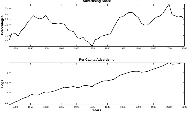
[image:13.612.114.500.83.320.2]

Years Per Capita Advertising

Figure 1.1: Advertising in Postwar U.S. economy. Panel 1. Advertising as share of GDP.

Panel 2. Per-capita real advertising. Coen’s annual data, sample from 1948 to 2005.

included among standard business cycle indicators. Appendix A lists the sources used to collect the data. The resulting database is novel in the literature, and is to our knowledge the only

up-to-date free-of-charge quarterly series for U.S. aggregate advertising.8 Our data report firms’

expenditures for advertisements in 7 media types, namely cable and network television, radio, newspapers, magazines and Sunday magazines, billboards, direct mail, and outdoor advertising. The sample starts in the first quarter of 1976 and ends in the second quarter of 2006 (122 quarters). In order to check whether the series provided is actually representative of all U.S. aggregate advertising expenditures, we compute the cumulative yearly expenditures from our data set and compare them with annual data for total advertising expenditures constructed by Robert Coen of Universal McCann; advertising experts consider this to be the most reliable source of data on aggregate advertising. In the considered sample, our series accounts on average for 30% of Coen’s

aggregate advertising, with a minimum of 25%, and an in-sample standard deviation of 2.95%.

Coen’s annual data are also useful in assessing the magnitude ofaggregate advertising. Figure

(1.1) plots the ratio of advertising over GDP (panel 1), which measures the relative importance of

advertising as a component of GDP, and per-capita real advertising expenditures (panel 2), which are commonly used in the literature as a measure of the number of advertising messages that reach

the consumer − i.e., a proxy for the intensity of advertising in the economy. The first statistics

fluctuate around 2.1% throughout the sample, with a maximum peak in year 2000, while the

second show a steady and strong upward trend, implying that the number of advertising messages per individual has constantly grown during the second half of the last century.

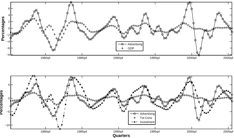
The novel series of quarterly data is used in figure (1.2) to represent the cyclical component of

8_{The U.S. Federal administration used to collect quarterly data for aggregate advertising, but it stopped after}

(14)

1980q4 1985q4 1990q4 1995q4 2000q4 2005q4 −8

−6 −4 −2 0 2 4 6

Percentages

Advertising GDP

1980q4 1985q4 1990q4 1995q4 2000q4 2005q4

−10 −5 0 5

Quarters

[image:14.612.115.496.88.314.2]

Percentages Advertising Tot Cons Investment

Figure 1.2: Advertising and the main Business Cycle Indicators. Quarterly figures. Data

sample from 1976q1 to 2006q2.

real advertising expenditures along with that of real GDP, real total consumption, and real fixed

private investment.9 _{Basically, the figure shows that (i) advertising is pro-cyclical; and that (ii) it}

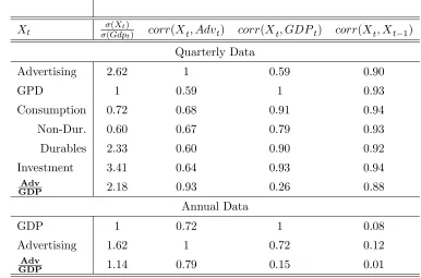
is more volatile than GDP and consumption and less so than investment. Table 1.1reports some

related statistics, which confirm these findings: advertising displays a high and positive correlation with GDP (0.59), and it is 2.62 times more volatile than GDP. In addition, it appears to be very

persistent over the cycle, with a point estimate of first-order autocorrelation of 0.89. Besides,

the positive correlation (0.26) between the advertising-GDP ratio and GDP itself suggests that

advertising cannot be simply assumed as a constant proportion of output.

Regarding the other aggregates, advertising displays the strongest correlation with total

con-sumption expenditures (0.68), and it has a very high standard deviation, with a point estimate 3.64

times higher than the one for consumption. Specifically, advertising is 4 times more volatile than non-durable consumption, slightly more volatile than expenditures in durable goods (the relative

standard deviation is equal to 1.12), and 23% less volatile than investment.

Since we have only a partial series of aggregate advertising expenditures, we check the robust-ness of the previous findings by computing the same statistics with Coen’s annual data. Results

are provided in the second panel of Table 1.1. Annual data confirm the quarterly evidence:

ag-gregate advertising is pro-cyclical − corr(Advt, GDPt) = 0.72 −, and more volatile than GDP−

σ(Advt)/σ(GDPt) = 1.62.

Finally, we analyse the dynamic cross-correlations between advertising, GDP, consumption,

9_{All the quarterly figures used in this section are in logs and per capita units. In figure (}_1.2_{), the cyclical}

(15)

[image:15.612.107.493.124.379.2]

Table 1.1: Second order moments

Xt _σσ₍_Gdp(Xt)_t₎ corr(Xt, Advt) corr(Xt, GDPt) corr(Xt, Xt−₁)

Quarterly Data

Advertising 2.62 1 0.59 0.90

GPD 1 0.59 1 0.93

Consumption 0.72 0.68 0.91 0.94

Non-Dur. 0.60 0.67 0.79 0.93

Durables 2.33 0.60 0.90 0.92

Investment 3.41 0.64 0.93 0.94

Adv

GDP 2.18 0.93 0.26 0.88

Annual Data

GDP 1 0.72 1 0.08

Advertising 1.62 1 0.72 0.12

Adv

GDP 1.14 0.79 0.15 0.01

[image:15.612.123.484.506.691.2]

Note:σ(.) is in-sample standard deviation. Annual data have been detrended using the BP(2,8)

Table 1.2: Dynamic cross correlations.

corr Xt,Gdpt+k

k -4 -3 -2 -1 0 1 2 3 4

Advertising 0.01 0.20 0.38 0.52 0.59 0.60 0.55 0.47 0.38

Consumption 0.16 0.39 0.62 0.81 0.91 0.90 0.78 0.58 0.35

Investment 0.27 0.54 0.76 0.91 0.93 0.84 0.66 0.42 0.18

corr(Xt,Advt+k)

Consumption 0.35 0.46 0.57 0.65 0.68 0.63 0.51 0.34 0.13

Non-Dur. 0.34 0.47 0.59 0.67 0.67 0.60 0.46 0.28 0.08

Durables 0.16 0.26 0.38 0.50 0.60 0.64 0.58 0.44 0.25

(16)

and investment. Dynamic correlations are useful in providing empirical evidence in order to sup-port or dismiss the idea that advertising can be a leading indicator of the cycle. As we see from

Table 1.2, advertising only slightly leads GDP: the cross-correlation coefficient is almost the same

at k=0 (0.59) and k=1 (0.60). Also, advertising appears to move contemporaneously with con-sumption (i.e., the strongest correlation occurs at k=0), while it strongly leads investment (higher correlations occur at k=-2 and k=-1). Overall, the dynamic cross-correlations seem to dismiss the idea that advertising can be used as a leading indicator of the cycle. The fact that advertising slightly leads GDP could be due to the fact that it moves with consumption, which itself has been

shown to slightly lead GDP in actual data.10

Overall, the main findings of this section can be summarised as follows:

• The amount of resources invested in advertising in the U.S. accounts for roughly 2% of GDP.

• Advertising is strongly procyclical and positively correlated with both consumption and

investment.

• Advertising is highly volatile, more volatile than GDP and consumption, but less volatile

than investment. Also, it is persistent over the cycle.

1.3 A DSGE model with Advertising

This section describes the model economy and displays the problems of households and firms. The market consists of a continuum of differentiated goods produced by monopolistically compet-itive producers that possess the technology to advertise their products. Advertising is assumed to

generate anurge to consume the advertised good. We obtain this effect by introducing advertising

as an argument of the utility function that is complementary to consumption (we support this

modelling strategy in section1.3.5). We then embed the modified utility function with advertising

into an otherwise standard dynamic stochastic growth model with no nominal or real friction, and we study the dynamics of this model in reaction to: (i) a shock to production technology; (ii) a shock to preferences; (iii) a shock to exogenous government spending; (iv) an idiosyncratic shock to the production of advertising.

1.3.1 The household and the role of advertising

We assume that a representative consumer exists with preferences defined for consumption and hours worked, which are described by the utility function:

U( ˜Ct, Ht) =E0

∞

X

t=0 βt

"

˜

Ct

(1−_σ₎

−1

1−σ −ξt

H_t1+φ

1 +φ

#

(1.1)

where ˜Ct is the consumption aggregate, Ht is the time devoted to work, and ξt is a preference

shock. The composite consumption aggregate ˜Ct is defined as follows:

˜

Ct =

 

1

Z

0

(ci,t+B(gi,t))

ε−1 ε _di

 

ε ε−1

(1.2)

10_{This evidence is not clear in our data, where the correlation between consumption and output is almost the}

(17)

whereε >1 is the pseudo-elasticity of substitution across varieties; gi,t is the goodwill associated

with goodi, where goodwill is meant to represent the stock of the firm’s advertising accumulated

over time; and B(·) is a decreasing and convex function controlling for the impact of goodwill on

consumer’s preferences, satisfyingB(0) =a≥ 0.11 We introduce the concept of goodwill because

several empirical studies have shown that advertising campaigns affect product sales for several

periods, evidence that seems robust across different goods, countries, and time periods.12

Building on Arrow and Nerlove (1962), we model the dynamic effect of advertising by assuming

that current and past advertising combine to create a reputation for a good, the producer’sgoodwill,

which is defined as the intangible stock of advertising that affects the consumer’s utility at timet,

as shown in (1.2). The stock of goodwill evolves according to the law of motion:

gi,t=zi,t+ (1−δg)gi,t−1 (1.3)

where zi,t is a firm’s investment in new advertising at time t and δg ∈ (0,1) is the depreciation

rate of the goodwill. The law of motion (1.3) implies that current sales could be affected not only

by current advertising expenditures, but also by past advertising, with a decreasing intensity over time.

In this setup, the positive link between the producer’s goodwill and sales operates through the

marginal utility of consumption. Notice that from (1.2) follows:

∂2C˜t

∂ci,t∂gi,t

∝ −1

ε(ci,t+gi,t)

−(1+ε)

ε B0(g_i,t)≥0 (1.4)

where the last inequality comes from the assumption that B(·) is decreasing in gi,t. This setup

reflects what is known in the literature as the persuasive role of advertising: advertisements create some added value for the good that would otherwise not exist. Consequently, the promoted good is worth more to consumers, as if it were a new or different good. The intuition behind this effect is that advertising creates dissatisfaction in the consumer about his current level of consumption.

The consumption aggregate (1.2) is modelled in the spirit of the ”catching up with the Joneses”

hypothesis of Abel (1990), or better, is based on the single-good habits version proposed by Ravn

Schmitt-Grohe and Uribe (2006).13

The rest of the model is standard. We assume that the representative consumer holds one

asset, the capital stockKt, which he rents to firms, and that he supplies labour services per unit

of time. Labour and capital markets are perfectly competitive, with a wage Wt paid per unit of

labour services and a rental rateRt paid per unit of capital. In addition, the consumer receives net

profits Πt from firms and pays lump sum taxesTt to finance the exogenous government spending.

Under these assumptions, the representative agent’s nominal budget constraint is defined as:

1

Z

0

pi,t(ci,t+ii,t)di≤WtHt+RtKt−₁+ Π_t−T_t (1.5)

11_{The consumption aggregate (}_1.2_{) is a Stone-Geary-type non-homothetic utility function. Depending on whether}

the termB(gi,t) is assumed to be positive or negative, the utility displays a saturation point or a subsistence level with respect to each variety consumed.

12_{In particular, see Clarke (1976) for an empirical study of the dynamic effects of advertising in the U.S. and}

Bagwell (2005) for a survey.

13_{As in the case of external habits, goodwill works in the utility as a negative externality for the consumer. With}

(18)

The utility maximisation problem for the representative consumer can be stated as a matter

of choosing the processes ˜Ct, Ht in order to maximise the utility function (1.1) subject to the

standard law of the motion of capital, i.e., Kt+1 = (1−δk)Kt +It, and the budget constraint

(1.5).14 Note that in our setup the consumer does not choose the desired goodwill, but instead

passively receives the whole amount of advertising determined by the firms.15 _{The first-order}

conditions for an interior maximum are:

˜

C−σ t

Pt

=λt (1.6)

λt =βE{λt+1[Rt+ (1−δk)]} (1.7)

ξtHtφ=Wtλt (1.8)

whereλt is the Lagrange multiplier associated with the budget constraint, andPt is the aggregate

price index. Equation (1.7) is the familiar Euler equation that gives the intertemporal optimality

condition, while equation (1.8) describes the labour supply schedule.

The optimality conditions (1.6), (1.7), and (1.8) mimic those of the standard neoclassical growth

model, but with the remarkable difference that the definition of the shadow price λt depends not

only on aggregate consumption but also on aggregate goodwill. Consequently, consumer’s decisions

about labour and investment are affected by the level of aggregate advertising.16

This mechanism plays a pivotal role in determining the general equilibrium results that we will explore in the next section. A partial equilibrium analysis is useful for understanding how adver-tising affects demand. Suppose, for instance, that adveradver-tising expenditures increase exogenously

for a sufficiently large fraction of firms. Given our assumptions, RB(gi,t)di decreases, and as a

consequence, the consumer’s shadow priceλt increases. Consider now the labour supply schedule

(1.8). An increase inλt implies that the agent values consumption more than leisure, since for any

given wage the marginal rate of substitution increases. Hence, the labour supply schedule shifts to the right, or the agent is willing to work more in order to consume more.

An increase in λt also affects the consumer’s saving decisions by changing the intertemporal

elasticity of substitution in the Euler equation (1.7). However, since (1.7) is a function of the ratio

of currentλt over future λt+1 marginal utility, the sign of the effect of higher advertising depends

on the relative response of current over future goodwill. In this simple example, the eventual effect

is easily predictable. The goodwill is an AR(1) process, and we assumed a one-time increase in

advertising: current consumption will increase. In general, an increase in advertising due to an exogenous shock, while unambiguously shifting the labour supply to the right, has an effect on the saving function that is determined by the dynamic response of expected future goodwill to a shock, which itself depends on several different general equilibrium effects that combine together. In particular, however, whenever the growth rate of the goodwill is positive, the consumer finds it

14_{To solve the maximisation problem, it is useful to write the budget constraint in the Lagrangian as a function}

of ˜Ct,It. Note that at the optimum,

1

R

0

pi,tii,tdi=PtItand

1

R

0

pi,tci,tdi=PtCt˜ − 1

R

0

pi,tgi,tdi.

15_{This feature distinguishes our model from Becker’s (1993)}_{complementary} _{theory of advertising. Following the}

Persuasive view of advertising, we assume that the agent passively receives the advertising signals without being aware of the effect they have on his preferences. On the contrary, in Becker (1993), the agent actively demands the informative content of advertising, since it raises the utility he gets from consumption.

16_{In particular, insofar as}_Ct_e _{has a negative first derivative with respect to the aggregate goodwill, then advertising}

(19)

more convenient to postpone his consumption, since he foresees that his marginal utility will be higher in the future. Conversely, when the growth rate of the goodwill is negative, the consumer

experiences anurge to consume and increases his demand for current consumption.

Overall, this analysis suggests that from the standpoint of a consumer, aggregate advertising can be interpreted as an exogenous state variable that modifies its own supply of labour and savings modifying, respectively, the elasticity of the wage and the intertemporal elasticity of substitution.

1.3.2 Firms

There is a continuum of firms indexed by i ∈ [0,1], each producing a differentiated product

that is sold as an item for consumption, an investment, or a government good.

The optimal demand function for consumption goods is the solution to the consumer’s problem

of minimising consumption expenditures subject to the aggregate constraint (1.2), i.e.,

ci,t = max

(

pi,t

Pt

−ε ˜

Ct−B(gi,t) ; 0

)

(1.9)

where

Pt =

 

1

Z

0 p1−ε

i,t di

 

1 1−ε

(1.10)

is the nominal price index. Equation (1.9) has two key implications for this paper, which we shall

explore in turn.

Firstly, the demand for consumption goods increases with the level of advertising. A positive

investment in zi,t raises the stock of goodwill gi,t, which in turns decreases B(gi,t), thus shifting

the demand function (1.9) to the right. The prediction of a positive relationship between sales and

advertising is in line with a large number of empirical studies about advertising at the firm level,17

and in our model derives from the assumption that advertising enters into the utility function. However, it is worth noting that this assumption is not arbitrary once we restrict our attention to models with Walrasian demand functions and perfect information. In this case, the only way that

advertising can enhance demand is through a modification of the preference relation.18

Secondly, the price elasticity of the demand diminishes with the level of advertising. Specifically,

the demand function (1.9) is composed of two terms: the first one, (Pi,t/Pt)

−ε _e

Ct with elasticity

ε, and the second one B(gi,t), which is inelastic. Overall price elasticity is then a combination

17_{Actually, a positive relationship between advertising and sales is one of the few non-controversial pieces of}

evidence regarding advertising. See Bagwell (2005), section 3.2, for more references.

18_{The argument proceeds by contradiction. First, recall that advertising according to our assumptions is not a}

(20)

between the elasticity of these two terms, and we can show that its value will depend on the relative importance of the goodwill over the total demand, i.e.,

η(ci,t, gi,t) =

_∂p∂ci,t_i,tp_c_i,ti,t =ε

1 +B(gi,t)

ci,t

(1.11)

In particular, notice that the elasticity of demand (1.11) is always smaller than the elasticity

of the demand without advertising, i.e., with gi,t = 0, since B(gi,t) is decreasing over gi,t. This

feature of the model replicates a well-known effect of advertising in the literature: firms advertise their products to develop consumers’ loyalty. The intuition is that advertising, although it does

not modify the quality of the advertised good, increases the differentiation among goodsperceived

by consumers. Thus, firms can use advertisements to manipulate the elasticity of the demand, thus increasing market power, and eventually profits.

The goods produced by firms are sold as consumption, investment, and government purchases. Unlike consumption, investments and government purchases are assumed not to be affected by

advertising.19 The assumption about the demand for investment goods fits naturally into our

setup because by assumption we modelled a positive effect of advertising on consumer’s willingness to consume, whereas investment represents the alternative option for the consumer who does not want to consume. The second assumption about government spending is conservative with respect to the results we will find, since it can be shown that modelling a positive effect of advertising on government expenditures would strengthen the effect of advertising on the aggregate dynamics.

Altogether, the demand for consumptionci,t, investment ii,t, and government expendituresfi,t

forms the total demand of firmiat timet, i.e.:

yi,t≡ci,t+ii,t+fi,t=

pi,t

Pt

−ε ˜

Ct+It+Ft

−B(gi,t) (1.12)

Accordingly, firm i chooses a price for sales and a level of advertising in order to maximise

the discounted flow of future profits subject to the constraint given by (1.12). The optimal policy

rules, which are derived formally in Appendix B, are:

pi,t =

ε1 + B(_ygi,t)

i,t

ε1 +B(_ygi,t)

i,t

−1

ϕt ≡µi,tϕt (1.13)

−(pi,t−ϕt)B0(gi,t) +Et[(1−δg) (νi,t+1rt,t+1)] =νi,t (1.14)

whereϕt is the marginal cost of production andνi,t is the marginal cost of producing new

adver-tising zi,t.

Equation (1.13) describes the familiar pricing policy in monopolistic competition models: the

firm exploits its monopolistic power by charging a positive markup µi,t over the marginal cost.

Unlike the standard case, µi,t is not constant but increases with the level of goodwill due to the

negative relation between price elasticity (1.11) and goodwill.

Equation (1.14) describes the optimal advertising policy. It states that the firm invests in

advertising until the marginal benefit from an extra dollar of advertising equals the marginal costs of producing it. Given the dynamic nature of goodwill, the marginal benefit on the LHS of

(1.14) has two components: the increase in current revenues associated with a marginal increase in

(21)

advertising, and the discounted opportunity cost of not producing tomorrow the surviving goodwill produced today.

According to (1.14), advertising is sensitive to variations in the conditions of both supply and

demand. On the one hand, reductions in marginal costs lead to higher investments in advertising. On the other hand, the marginal benefit of advertising depends on markup that is positively

affected by aggregate demand (see equation 1.13). Hence, any exogenous increase in the demand

simultaneously raises markup and advertising.

Besides, note that (1.13) and (1.14) together imply that advertising and price-setting are

complementary policies, in accordance with the theory of optimal advertising as the outcome of

firms playing a supermodular game, as shown in Tremblay (2005).20

Interestingly, we can establish an equivalence result between the optimal advertising policy

(1.14) and the seminal Dorfman-Steiner (1954) theorem about firms’ optimal spending on

adver-tising, which states that the optimal budget for advertising expenditures is equal to the ratio between the elasticity of the demand with respect to advertising and the elasticity of demand with respect to price. The equivalence result is contained in the following proposition.

Proposition 1. Let the demand function for firm ibe defined as in (1.12), and denoteηg,t(i) and

η∗

p,t(i) as the elasticity of the demand with respect to goodwill and the elasticity of the demand with respect to price, respectively. Then, the optimal level of goodwill for firm i will be a proportion of the ratio of ηg,t(i) over ηp,t∗ (i).

Proof. First notice that from (1.12) follows:

−B0

(gi,t) =ηg,t(i)

yi,t

gi,t

Using this result into (1.14) to substitute outB0

(gi,t) and rearranging, it yields:

gi,t

yi,t

=ηg,t(i)

pi,t−ϕt

νi,t−Et[(1−δg) (νi,t+1rt,t+1)]

or, substituting outpi,t using the optimal pricing rule (1.13),

gi,t

yi,t

= ηg,t(i)

η∗

p,t(i)

Ωt,i (1.15)

where Ωi,t = _ν_i,t−Et[(1−δgϕ)(tνi,t+1rt,t+1)] and η

∗

p,t(i) = (η(yi,t, pi,t)−1). Thus, the optimal goodwill

intensity is proportional to the ratioηg,t(i)/η∗p,t(i).

It is straightforward to see that equation (1.15) is a general result that nests the

Dorfman-Steiner theorem as a particular case whenδg = 1 andνi,t =ϕi,t, i.e., the goodwill fully depreciates

in each period, and firms use the same technology to produce goods and advertising.

(22)

1.3.3 Advertising and consumption persistence

Another result embedded in equation (1.15) is that advertising generates persistence in the

dynamics of consumption. To prove this claim, first note that at the symmetric equilibrium:21

η∗

p,t(i) =η

∗

p,t(j),ηg,t(i) = ηg,t(j), andνi,t =νj,t ∀i, j. Then, rewrite equation (1.15) as:

gi,t= Φtyi,t (1.16)

Using (1.16) lagged one period to work outgi,t−₁ from the law of motion of goodwill (1.3), and

plugging the result into the demand function (1.9) to work outgi,t, we obtain:

yi,t =

pi,t

Pt

−ε

e

Ct+It+Ft

+ψ(Φt, yi,t−₁, zi,t) (1.17)

whereψ(·) is a non-linear function with a non-negative partial derivative with respect to the last

two arguments.22

Equation (1.17) reveals that the demand faced by each producer depends on past sales, as

in customers market models or models that include habits of consumption.23 _{This result is}

de-termined by two properties of our setup: (i) the assumption that the consumer’s preferences are affected by advertising; and (ii) the dynamic nature of the goodwill. As noted in the introduction, advertising naturally rationalises the presence of consumption persistence within the theory of rational consumer and profit-maximising firms. Compared with other models that have explained consumption persistence, the advantage of using advertising is that persistence is endogenously de-termined at equilibrium based on the optimising behaviour of firms, once we explicitly incorporate into the model the observable and well-known phenomenon of advertising, instead of being derived

from anad hoc assumption like ”the costumers” in the market or ”the habits” in the utility.

1.3.4 The Symmetric Equilibrium

In this model the market for production factors is perfectly competitive, and all firms share the

same production technology. Thus, all firms face the same marginal cost.24 _{Moreover, all goods}

have the same pre-advertising elasticity of substitution, i.e.,ε. These two conditions imply together

that a symmetric equilibrium exists where all firms set the same price, produce the same quantities,

and invest the same amount of resources in advertising.25 _{In addition, the equilibrium (common)}

price of goods is normalised to unity in each period, i.e., pt = 1 ∀t. Thus, all other prices in the

model (e.g., wage, rental rate) are expressed in terms of contemporaneous consumption.

LetXt be the vector of all endogenous variables,26then the symmetric equilibrium is a process

{Xt}

∞

t=0that satisfies: (1.6)-(1.8), (1.13)-(1.14), plus the production function of consumption goods

and advertising, the optimal factors demand for productions,27 the laws of motion of capital and

goodwill, the market clearing condition on the goods market, Yt =Ct +It+Ft, and the market

clearing condition on the labour market, Ht =Hp,t+Ha,t.

21_{See section}_1.3.4_.

22_{This follows immediately from the fact that}_B₍_·_{) is assumed to be strictly decreasing together with the fact that}

non-negative optimal advertising requires Φt>0.

23_{For more about this issue, see Ravn, Schmitt-Groh´e and Uribe (2006), and the ”habit persistence” entry of the}

Palgrave Economic Dictionary, written by Schmitt-Groh´e and Uribe (2006).

24_{The reader can check this by inspecting the RHS of equation (}_1.7.3_).

25_{This equilibrium requires the extra assumption that the initial stock of goodwill is the same across firms.} 26_{Specifically,}_Xt _{= (}_{λt, Gt, µt, Zt}_{, Ht, Ha,t, Hp,t, Ct, Kt, It, Yt, Rt}_{, Wt, Qt,t}

(23)

1.3.5 Advertising in Utility Function: Functional Forms Assumptions

In order to fully specify the utility function, we need to parameterise the function B(·) in a

way that satisfies all assumptions made so far (see equation (1.2) and the following discussion). In

addition, we are interested in some specification of B(·) that nests market-enhancing and

spread-it-around advertising.

In the following, we assume that the functionB(gi,t) is defined as:

B(gi,t)≡S(gi,t) +γ

1

Z

0

(1−S(gi,t))di with γ ∈ [0,1] (1.18)

where

S(gi,t)≡ 1 1 +θgi,t

(1.19)

It is easy to verify that the function (1.19) is strictly decreasing and convex in goodwill. More

importantly, the goodwill in (1.18) enters in quasi-difference from its market average, meaning that

the effectiveness of firm’s advertising on its own demand will depend on the level of advertising of

competitors.28

Now, we consider in detail the role of γ. At symmetric equilibrium, (1.18) and (1.19) imply:

B(Gt)≡

1 +γθGt

1 +θGt

If γ = 1, then B(gi,t) = 1. Thus, the aggregate goodwill disappears from the marginal utility

of consumption (see equations (1.6) and (1.2)), and does not directly affect the representative

consumer’s decisions about labour supply (1.7) and savings (1.8), and therefore the

spread-it-around hypothesis holds. In this case, the effect of advertising on the whole economy is easily predictable. It absorbs resources without enhancing demand, and it has no direct effect on prices. Thus, it is a deadweight loss both for firms and for the consumer. Note that firms are still employing resources to advertise their products because in the non-cooperative solution, they do not internalise the effect of their decisions on the mean level of advertising. As a result, they keep wasting money in an unproductive way while the effect of their advertisements on their own demand is offset by other firms’ advertising.

Ifγ = 0 the goodwill enters in level in the utility function. Accordingly, each firm’s advertising

affects the marginal utility of its product no matter what the other firms do. In this case advertising directly affects consumption, labor, investment, and firms’ markup, and its overall effect in the

general equilibrium will be the object of the analysis in next section 1.4. Finally, any value of

γ ∈(0,1) implies a convex combination between the two extreme cases (complete spread-it-around

vs. market enhancing).

A consideration apart deserves the choice of S(·). Equation (1.19) implies that the marginal

utility of consumption is bounded (hence we will refer to it as ”bounded marginal utility”).29 Due

to this bound, in the demand function (1.9) there exists a maximum price above which the demand

is zero: when the price is too high the marginal benefit of consuming that good is smaller than its cost, and the consumer drops it from his basket of purchases. In this fashion, firms have incentive to advertise their products for reducing the bound. In the absence of advertising, the bound is constantly equal to 1, while with advertising the bound depends on the level of goodwill, whose

28_{This formulation implies that advertising is combative.}

29_{As a matter of fact, preference featuring bounded marginal utility have been already used in the literature. See}

(24)

effect is larger with largerθ. Hence, this parameter is interpreted as a measure of the effectiveness of advertising in manipulating consumer’s tastes.

1.4 Impulse-Response Analysis

This section considers a log-linear approximation of the model’s policy functions in the neigh-bourhood of the non-stochastic steady state. Rational expectations are solved to obtain the dynamic responses of endogenous variables as functions of state variables. We characterise the response of the model’s variables to several exogenous shocks, namely: a technology shock (figure

1.3), a preferences shock (figure 1.4), a shock on exogenous government spending (figure 1.5), and

an idiosyncratic shock to the production function of advertising (figure 1.6).

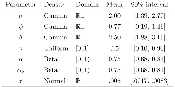
To compute the impulse-response functions (hereafter IRFs), we need to assign values to the

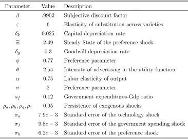
parameters {β, σ, φ, Ξ, ε, θ, α, ρz, ρa, ρf, ρh, σh, σa, σf, δg, δk, γ}. The parameters that are

standard in real business cycle (hereafter RBC) models are calibrated using the values commonly used in the literature, while the others are chosen such that steady states of model variables match

selected long-run moments of U.S. postwar data. In particular, the discount parameterβ is set to

(1.04)−.25_{, implying a yearly nominal interest rate of about 4%. The depreciation rate of capital}

δk is equal to 2.5% per quarter, and the gross elasticity of substitution across varieties is equal to

6. Following Prescott (1986), the preference parameter Ξ is chosen to ensure that in the steady

state, the consumer devotes 1/4 of his time to labour activities. Following Ravn, Schmitt-Groh

and Uribe (2006), we set the intertemporal elasticity of substitution to 0.5, the labour elasticity of

output α to 0.75, the Frisch elasticity of labour supply to 1.3, and the government

expenditures-GDP ratio sf to 0.12. These restrictions imply that the preference parametersσ andφare 2 and

0.77, respectively, and the steady state labour share is 0.71.30

The values of advertising related parameters have been assigned using the following strategy.

The goodwill depreciation rate has been fixed to 0.3, implying that the half life of goodwill stock is

about two quarters. This value is consistent with the empirical evidence provided in Clarke (1976): the effect of advertising on the firm’s demand basically vanishes after one year. As a benchmark

case, we set the parameterγ to zero, while the intensity of advertising in the utility function θis

chosen such that conditional to all other parameters, the steady-state value of the advertising over

GDP ratio is equal to 2.27%, consistent with the U.S. average over the period 1948-2005.31

The autoregressive parameters for all the endogenous process have been set to 0.95. This number is intermediate among the values normally used in the RBC literature. For the simulations, following Rebelo and King (1998) and Collard (2006), we set the standard deviations of technology

shock σa and government expenditures shock σf to 0.0079 and 0.0089, respectively. Finally, the

standard deviation of the preference shock σh is chosen such that the volatility of hours worked

in the model matches its empirical counterpart of 0.91%.32 The time period in the model is one

30_{In our framework, the steady state labour share denoted by}_sh _{takes the following form:}

sh = W(Hp+Ha)

Y

= αµ−1_{1 +}Ha Hp

so that the usual relationship between the intensity of labour in the production function and the labour share no longer necessarily holds. Note that in the last equation,µdenotes the average long run markup.

31_{This number refers to the ratio of advertising expenditures to net GDP, where exports are subtracted from GDP}

because exported goods are not sold based on domestic advertising.

(25)

[image:25.612.119.485.108.379.2]

Table 1.3: Calibration

Parameter Value Description

β .9902 Subjective discount factor

ε 6 Elasticity of substitution across varieties

δk 0.025 Capital depreciation rate

Ξ 2.49 Steady State of the preference shock

δg 0.3 Goodwill depreciation rate

φ 0.77 Preference parameter

θ 2.54 Intensity of advertising in the utility function

α 0.75 Labor elasticity of output

σ 2 Preference parameter

sf 0.12 Government expenditures-Gdp ratio

ρa, ρh, ρg, ρz 0.95 Persistence of exogenous shocks

σa 7.9e−3 Standard error of the technology shock

σf 9.8e−3 Standard error of the government spending shock

σh 6.2e−3 Standard error of the preference shock

quarter. Table 1.3 summarises the set of calibrated parameters.

We plot the IRFs for different values of the spread-it-around parameter γ, and we use the

associated model economy where advertising is banned as a benchmark to evaluate the impact of

advertising. The IRFs appear in Figures (1.3) − (1.6), and we will emphasise a number of these

results.

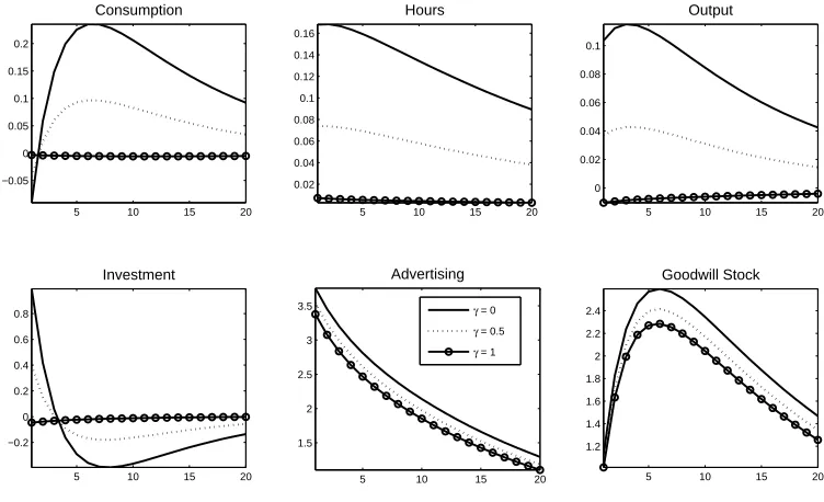
First, advertising responds positively to any shock considered. This result follows directly

from equation (1.16), which establishes a positive relationship between aggregate goodwill and

aggregate demand. Whenever a shock increases demand, the marginal benefit of goodwill also increases, pushing firms to invest more in advertising. In particular, of the shocks considered,

advertising reacts mostly to the technology shock, as is apparent by comparing figures (1.3) and

(1.4). The response of advertising to a 1% technology shock is twice as large as the response to a

1% preference shock. This is due to the double effect of an unexpected increase in productivity; the firm revises its advertising spending on the one end because the demand increases, and on the other end because the marginal cost of advertising diminishes. Note that this second effect is further amplified by the dynamic nature of advertising, which modifies the optimal plan of

producing advertising to stock future goodwill.33

Second, advertising in the model is pro-cyclical, as it becomes apparent comparing the IRFs

of advertising and output in figures (1.3) − (1.6). After each shock, the pairs of IRFs display

the same sign both at impact and afterward during the transition back to the steady state, thus replicating the positive correlation between advertising and GDP observed in real data. Note that

33_{Clearly, in the event of a transitory positive technology shock, producing advertising today becomes cheaper}

(26)

0 5 10 15 20 0.5 0.6 0.7 0.8 0.9 1 1.1 1.2 1.3 Consumption

γ = 0 γ = 0.5 γ = 1 bench

0 5 10 15 20

0.1 0.2 0.3 0.4 0.5 0.6 0.7 0.8 Hours

0 5 10 15 20

0.8 1 1.2 1.4 1.6 Output

0 5 10 15 20

0 1 2 3 4 5 6 7 8 Investment

0 5 10 15 20

0.5 1 1.5 2 2.5 3 3.5 4 Advertising

0 5 10 15 20

[image:26.612.126.497.81.315.2]

1 1.2 1.4 1.6 1.8 2 2.2 2.4 2.6 Goodwill

Figure 1.3: Impulse Response Functions to technology shock. Each plot displays percent deviation

from steady state of the corresponding variable in response to a 1% increase in the rate of productivity.

this feature of the model is independent of the value assigned to γ.34

Third, spread-it-around and market-enhancing advertising play two very different roles in the

aggregate dynamics. When γ = 1 (spread-it-around), the IRFs of the main economic aggregates

essentially coincide with the benchmark ones (compare dashed versus circle lines): i.e., the effect of advertising on the aggregate becomes negligible. As intuition suggests, in this case advertising does not influence consumer’s decisions, and its effect on the aggregate dynamics is determined only by the excess of labour demand that results from producing advertising. The numerical analysis shows that such an effect is negligible since the absorbtion of resources due to advertising is too small to affect the other aggregates in a relevant way. Hence, the conjecture of Simon and Solow is confirmed: under the spread-it-around hypothesis, advertising is irrelevant in the aggregate.

Oppositely, whenγ6= 1 (market-enhancing), advertising operates on the aggregate dynamics as

a mechanism that amplifies and propagates the effects of exogenous shocks (compare the continuous

versus dashed lines), and the effect turns out to be stronger when γ is lower (continuous versus

dotted lines). The effect of advertising on the labour supply is most important.35 Despite the

fact that wages are lower at equilibrium than in the benchmark model, the upward pressure that

advertising puts on the supply of labour is so strong that worked hours increase.36 This mechanism

is called the work and spend cycle (Schor, 1992), and it has been empirically supported by Brack

and Cowling (1983) for the U.S., and by Fraser and Paton (2003) for the UK.

As a result of the higher level of hours worked, production increases, and the response of output to any shock considered is stronger than the benchmark. The effect of advertising appears

34_{It has often been argued in the literature that the correlation between GDP and advertising is not a relevant}

statistic to the disentangling of market-enhancing advertising from spread-it-around advertising. This also remains true in our model.

35_{See Molinari and Turino 2007 for a detailed analysis.}

(27)

0 5 10 15 20 0.2 0.25 0.3 0.35 0.4 0.45 0.5 Consumption

γ = 0 γ = 0.5 γ = 1 bench

0 5 10 15 20

0.2 0.3 0.4 0.5 0.6 0.7 0.8 0.9 1 Hours

0 5 10 15 20

0.35 0.4 0.45 0.5 0.55 0.6 0.65 0.7 Output

0 5 10 15 20

0 0.5 1 1.5 2 2.5 3 3.5 Investment

0 5 10 15 20

0.4 0.6 0.8 1 1.2 1.4 1.6 1.8 2 Advertising

0 5 10 15 20

[image:27.612.123.496.81.316.2]

0.4 0.5 0.6 0.7 0.8 0.9 1 1.1 Goodwill Stock

Figure 1.4: Impulse Response Functions to preferences shock. Each plot displays percent deviation

from steady state of corresponding variable in response to a 1% decrease in the preference shock.

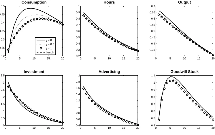
quantitatively relevant when γ = 0. Figure (1.6) shows that an unexpected 1% increase in the

productivity of advertising affects fluctuations in a non-negligible way; consumption increases by

0.25%, output by 0.12%, investment by 1.07%, and labour by 0.18%.37

Overall, the analysis of the aggregate dynamics reveals that demand-shifting advertising works as a built-in mechanism of the transmission of exogenous shocks. The case of a positive technology shock is particularly interesting in light of the RBC literature. Intuitively, an unexpected increase

in productivity leads to a higher level of desired goodwill.38 In turn, a higher level of goodwill

implies an upward shift in the demand of consumption goods, according to (1.17). Hence, after a

technology shock, the level of the aggregate demand increases not only because of the traditional transmission channels (higher wage and higher present value of wealth), but also because of the higher spending on advertising, which makes the consumer willing to consume more for any given price. In the RBC literature, it has often been argued that technology shocks cannot generate business cycles such as those observed in actual data. We suggest that the extra propagation

channel provided by advertising could help to reconcile the theory with the data. Section 1.5will

test this assertion.

Lastly, we want to emphasise the behaviour of consumption, whose dynamics in the model with respect to the benchmark display a lower response to the impact of the shock, but a larger, hump-shaped impulse response function during the transition. Given that by assumption advertis-ing raises the marginal utility of consumption in the model, the relative reduction of consumption at impact may not be intuitive and deserves further explanation. The basic intuition is that with advertising the consumer experiences temporal variations in the intertemporal elasticity of sub-stitution, which determines the relative reduction of consumption with respect to the benchmark

37_{Recall that advertising in the model is not a component of the output, which is defined as consumption plus}

investment and government spending.

(28)

5 10 15 20 −0.09

−0.08 −0.07 −0.06 −0.05

Consumption

γ = 0 γ = 0.5 γ = 1 bench

5 10 15 20

0.02 0.025 0.03 0.035 0.04 0.045

Hours

5 10 15 20

0.01 0.015 0.02 0.025 0.03 0.035

Output

5 10 15 20

−0.12 −0.1 −0.08 −0.06 −0.04 −0.02

Investment

5 10 15 20

0.03 0.04 0.05 0.06 0.07 0.08

Advertising

5 10 15 20

0.025 0.03 0.035 0.04 0.045 0.05 0.055 0.06

[image:28.612.118.498.81.315.2]

Goodwill Stock

Figure 1.5: Impulse Response Functions to government spending shock. Each plot displays

percent deviation from steady state of corresponding variable in response to a 1% shock on government spending.

economy. To see this point, it is useful to rewrite the log-linearised Euler Equation in terms of expected consumption growth, that is:

Et{∆bct+1}= (1−γ)ηc,gEt{∆bgt+1}+ ηc,p

ε

1

σEt{brt+1} (1.20)

where ηc,p and ηc,g are, respectively, the steady state demand elasticity with respect to price

and goodwill. According to (1.20), aggregate advertising modifies the savings decision along two

different dimensions. On the one hand, since the elasticity ηc,g is positive (the first term on the

RHS of (1.20), expected variations in the stock of goodwill modify the expected consumption

growth in the same direction. Intuitively, the consumer correctly anticipates the effect of future goodwill on the utility of future consumption and modifies the degree of consumption smoothness

over time accordingly. Clearly, the effect is stronger for lowerγ, since for values ofγ that approach

1, the evaluation of future utility becomes independent from the level of goodwill. On the other hand, the elasticity of expected consumption growth to the interest rate is lower than that used in

the benchmark model (second term in the RHS of 1.20), since the long run price elasticity ηc,p is

lower than the benchmark oneε.39 Hence, if interest rate and goodwill growth respond to a shock

in the same direction, the two effects tend to offset each other, and the overall impact will depend on which one prevails.

In our calibrations, the first effect dominates the second, making the response of consumption to a shock larger than in the benchmark model. This feature of the model becomes apparent upon inspecting the behaviour of investment. In all the cases considered, the IRF of investment

39_{Overall, since the impulse response function of the goodwill stock is hump-shaped, during the transition to the}

(29)

5 10 15 20 −0.05

0 0.05 0.1 0.15 0.2

Consumption

5 10 15 20

0.02 0.04 0.06 0.08 0.1 0.12 0.14 0.16

Hours

5 10 15 20

0 0.02 0.04 0.06 0.08 0.1

Output

5 10 15 20

−0.2 0 0.2 0.4 0.6 0.8

Investment

5 10 15 20

1.5 2 2.5 3 3.5

Advertising

5 10 15 20

1.2 1.4 1.6 1.8 2 2.2 2.4

Goodwill Stock

[image:29.612.118.494.86.315.2]

γ = 0 γ = 0.5 γ = 1

Figure 1.6: Impulse Response Functions to a shock on advertising production function. Each

plot displays percent deviation from steady state of corresponding variable in response to a 1% shock on the production function of advertising.

is stronger than the benchmark one up to the quarter in which the goodwill peaks. This effect is particularly interesting because it shows that contrary to the conventional wisdom, a positive link between consumption and advertising does not necessarily need to be associated with a crowding-out effect on investment. In fact, once we account for the dynamic effect of advertising and let the supply of labour be endogenously determined by the consumer, an equilibrium in which consumption, hours and investment all increase is indeed possible.

1.5 Model Estimation

This section estimates the DSGE model with advertising using a quarterly time series of U.S. macroeconomic data and a Bayesian estimation method. The data sample goes from the first quarter of 1976 to the second quarter of 2006, the interval over which we have data on aggregate advertising.

Bayesian estimation is preferred over other techniques for several reasons. First, it naturally accommodates the unobservable goodwill in the estimation algorithm, which is a crucial variable for estimating advertising related parameters. Second, it is preferred to Maximum Likelihood estimation because we want to pin down model parameters exploiting combined information from business cycle frequency data and long-run moments of the data, as we showed that advertising

also has a relevant effect in the long run.40 Bayesian priors are a convenient tool for including extra

information in the estimation. Third, the effect of advertising spreads in the economy through various transmission channels that can only be assessed completely by computing the general

equilibrium solution of the model, as we showed in section 1.4. Therefore, any estimation that