OFFPRINT
Scaling properties of excursions in heartbeat
dynamics
I. Reyes-Ram´
ırez
and
L. Guzm´
an-Vargas
EPL,
89
(2010) 38008
T
ARGET YOUR RESEARCH
WITH
EPL
Sign up to receive the free EPL table of
contents alert.
February 2010
EPL,89(2010) 38008 www.epljournal.org
doi:10.1209/0295-5075/89/38008
Scaling properties of excursions in heartbeat dynamics
I. Reyes-Ram´ırez1,2and L. Guzm´an-Vargas1(a)
1Unidad Profesional Interdisciplinaria en Ingenier´ıa y Tecnolog´ıas Avanzadas, Instituto Polit´ecnico Nacional
Av. IPN No. 2580, L. Ticom´an, M´exico D.F. 07340, M´exico
2Escuela Superior de F´ısica y Matem´aticas, Instituto Polit´ecnico Nacional - Edif. No. 9 U.P. Zacatenco,
M´exico D.F., 07738, M´exico
received 6 October 2009; accepted in final form 19 January 2010 published online 19 February 2010
PACS 87.19.Hh– Cardiac dynamics
PACS 89.20.-a– Interdisciplinary applications of physics
PACS 89.75.Da– Systems obeying scaling laws
Abstract– In this work we study the excursions, defined as the number of beats to return to a local mean value, in heartbeat interval time series from healthy subjects and patients with congestive heart failure (CHF). First, we apply the segmentation procedure proposed by Bernaola-Galv´an
et al. (Phys. Rev. Lett., 87 (2001) 168105), to nonstationary heartbeat time series to identify
stationary segments with a local mean value. Next, we identify local excursions around the local mean value and construct the distributions to analyze the time organization and memory in the excursions sequences from the whole time series. We find that the cumulative distributions of excursions are consistent with a stretched exponential function given by g(x)∼e−aτb, with
a= 1.09±0.15 (mean value±SD) andb= 0.91±0.11 for healthy subjects anda= 1.31±0.23 and
b= 0.77±0.13 for CHF patients. The cumulative conditional probability G(τ|τ0) is considered
to evaluate if τ depends on a given interval τ0, that is, to evaluate the memory effect in
excursion sequences. We find that the memory in excursions sequences under healthy conditions is characterized by the presence of clusters related to the fact that large excursions are more likely to be followed by large ones whereas for CHF data we do not observe this behavior. The presence of correlations in healthy data is confirmed by means of the detrended fluctuation analysis (DFA) while for CHF records the scaling exponent is characterized by a crossover, indicating that for short scales the sequences resemble uncorrelated noise.
Copyright cEPLA, 2010
Introduction. – Many biological systems exhibit complex fluctuations which are related to a large number of mechanisms participating across multiple time scales [1]. The characterization of these fluctuations is important to understand the internal dynamics of the systems. In this context, many studies have reported that the output of many biological systems which exhibits complex fluctuations can be characterized by the presence of scaling and fractal properties [2,3]. In recent years, many studies have focused on statistical properties of heartbeat interval sequences. It is well known that healthy heartbeat dynamics displays fluctuations characterized by a 1/f behavior with long-range correlations and a broad multifractal spectrum [2,4]. Closely related with these findings, the interbeat interval time series are described as extremely patchy and nonstationary, with very irregular fluctuations. An important aspect of the
(a)E-mail:[email protected]
interbeat variability and of other physiologic signals is that healthy systems have complex self-regulating mechanisms operating over multiple time scales and may generate signals that have scaling properties. Recently, methods from statistical mechanics and nonlinear dynam-ics have revealed that some scaling structures and complex variability observed under healthy conditions are altered by disease and aging [2,5–10]. A recent study to detect local stationary segments of heartbeat interval time series [11] revealed that the distribution of these stationary segments follows a power law behavior and the scaling exponent, which characterizes the distribution, is the same for healthy and heart failure groups. These findings indicate that this scale-invariant structure is not a simple consequence of long-range correlations [11] displayed by the system and that the nonstationarity is an intrinsic property related to neuroautonomic control and external perturbations. From a physiologic point of view, the presence of local stationary segments can be
I. Reyes-Ram´ırez and L. Guzm´an-Vargas
understood as the capability of the system to preserve an approximated constant value but for a limited period of time. It is also argued that, according to the homeostasis principle, biological systems tend to maintain a constant output in spite of continual perturbations [12]. Indeed, fluctuations or variations around certain value are a common characteristic of some physiologic signals in agreement with the mentioned homeostasis principle. Statistical analysis of excursions, which are defined as the period of time employed by a walker to return to its average value, may be important to the assessment of the capability of the system to preserve a mean output value. The problem of the first return time has been studied in contexts like financial index, correlated-disordered chains, intermittency, seismic activity and simulated noise [13–18]. There are also important results of zero crossing probabilities for Gaussian long-term correlated data [19]. In this work we focus our attention on the statistical properties of local excursions within the context of nonstationary heart rate time series. We observed that excursions for stationary segments lead to a class of exponential distributions which are characterized by different parameters for healthy subjects and heart failure patients. The paper is organized as follows: in the second section, we briefly describe the segmentation algorithm and the detrended fluctuation analysis method. In the third section, the results of the statistics of excursions are described. Finally, some concluding remarks are given in the last section.
Methods. –
The segmentation algorithm. We briefly explain
the segmentation method proposed by Bernaola-Galv´an
et al.[11] to detect stationary segments in a nonstationary
signal.
– A slider pointer is considered to calculate the statis-tics t=µr−µl
SD , where μr and μl are the mean of the values on the right and left, respectively. SD is the
pooled variance give by SD= [((Nl−1)s2l+ (Nr−
1)s2
r)/(Nl+Nr−2)]1/2(1/Nl+ 1/Nr)1/2, where sl
and sr are the standard deviation of the two sets,
andNl and Nr are the number of points in the two
sets.
– The quantity t is used to separate two segments with a statistically different mean. A significance level is applied to cut the series into two new segments (typically set to 0.95), as long as the means of the two new segments are significantly different from the mean of the adjacent segments [11,20].
– The process is applied recursively until the signif-icance value is smaller than the threshold, or the length of the new segment is smaller than a minimum ℓ0. For details in the implementation of the algorithm
see [20].
Correlations. The power spectrum is the typical
method to detect autocorrelations in a time series. For example, consider a stationary stochastic process with autocorrelation function which follows a power lawC(s)∼
s−γ, wheresis the lag andγ is the correlation exponent,
0< γ <1. The presence of long-term correlations is related
to the fact that the mean correlation time diverges for infinite time series. According to the Wiener-Khintchin theorem, the power spectrum is the Fourier transform of the autocorrelation function C(s) and for the case described above, we have the scaling relationS(f)∼f−β,
where β is called the spectral exponent and is related to the correlation exponent byγ= 1−β. One method which is particularly suited to analyze nonstationary signals is the detrended fluctuation analysis (DFA), which was intro-duced to quantify long-range correlations in the heartbeat interval time series and DNA sequences [21,22]. The DFA is described as follows: First, we integrate the original time series to get,y(k) =k
i=1[x(i)−xave], where xave is the
global mean; the resulting series is divided into boxes of sizen. For each box, a straight line is fitted to the points, yn(k). Next, the line points are subtracted from the
inte-grated series, y(k), in each box. The root mean square fluctuation of the integrated and detrended series is calcu-lated by means of F(n) =
1
N
N
k=1[y(k)−yn(k)]2, this
process is taken over several scales (box sizes) to obtain a power law behavior F(n)∼nα, with α an exponent,
which reflects self-similar and correlation properties of the signal. It is known thatα= 0.5 corresponds to white noise (noncorrelated signal),α= 1 means 1/f noise andα= 1.5 represents a Brownian motion.
Results. – We analyze heartbeat interval time series from two groups: 16 healthy subjects and 11 patients with congestive heart failure [23]. We considered RR interval sequences with approximately 3×10⁴beats corresponding
to 6 diurnal hours of ECG records. This database is an extended set of records which have been used in previous studies [9,10,23].
Distributions of local excursions. First, we apply
the segmentation procedure to interbeat interval time series to detect stationary segments. Figure 1(a) shows a representation of the segmentation procedure to the data from one healthy subject. In our study we used ℓ0= 50 as the minimum segment length. As it was reported
by Bernaola-Galv´an and coworkers [11], the cumulative distribution of stationary segments with local mean follows a power law,
G(> ℓ)∼ℓ−δ, (1)
with δ≈2.2 for healthy and heart failure groups [11]. Next, we calculate the excursions return times for each stationary segment with respect to the local mean. More specifically, we identify an excursion with sizeτ ifxj>x¯
and xj+τ>x¯ while xi>x¯ for j < i < j+τ or conversely
xj<x¯ and xj+τ<x¯ while xi<x¯ for j < i < j+τ (see
Scaling properties of excursions in heartbeat dynamics
Fig. 1: Representative case of the segmentation procedure for a nonstationary signal from a healthy subject (a). (b) As in (a) but for a magnification of the interval in (a). (c) Magnification of (b) to illustrate the excursion identification.
segments, we verify if the distribution from one segment corresponds to the same distribution of any other segment. In fig. 2(a) representative cases of excursion distributions from segments with small, intermediate and large length ℓare depicted. We observe that for the large segment the statistics is better than for distributions from intermediate or small length, but in the three cases a similar functional form is identified. We formulate the question whether any pair of stationary segments, regardless of their length, lead to distributions with the same functional behavior. The Kolmogorov-Smirnov (K-S) test is used to accept or reject the null hypothesis that any pair of segments have the same distribution. We computed thep-value between distributions from all the pairs of stationary segments detected in the signal.
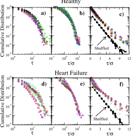
In figs. 2(b) and (c), we present the statistics of the results obtained from the application of the K-S test to healthy and CHF groups. We observe that, for both datasets and at 5% level of significance, in most of the cases we accept the null hypothesis that any two segments have the same distribution, suggesting that one can pool the data from all segments to improve the statistics. Now, we consider the cumulative distribution of excursion sequences from all the segments G(> τ). As shown in fig. 3(a), the distributions from the healthy group show a similar behavior with a different decaying rate (see next paragraph for a quantitative comparison). However, if one normalizes the excursions, that is, we divide the excursion size by its standard deviation, all the cases collapse onto a single curve, suggesting that they follow the same functional form (fig. 3(b)). A more detailed observation of these distributions indicates that they are consistent with a stretched exponential function given by
g(τ)∼e−aτ
b
, (2)
0 0.2 0.4 0.6 0.8 1
p-value 0
0.2 0.4 0.6 0.8 1
n
oit
u
bi
rt
si
D
e
vit
al
u
m
u
C
0.2 0.4 0.6 0.8 1
p-value
Healthy Heart Failure
100 101 102
Excursion size τ
0.01 0.1 1
no
it
ub
irt
si
D
ev
it
al
u
mu
C
l=120 l=420 l =900
b) c)
a)
Fig. 2: (Colour on-line) (a) Cumulative distribution of excur-sion sequences obtained from segments with different length
ℓ. We show the cases for ℓ= 120,420,900 from one healthy subject. (b), (c) Cumulative distribution ofp-values from the application of the Kolmogorov-Smirnov test to excursion distri-butions from all the pairs of stationary segments detected in healthy and CHF subjects. We find that, at 5% level of signifi-cance, for most of the cases we cannot reject the null hypothesis that any pair of segments have the same excursion distribution, suggesting that we can pool data from all the segments and improve the statistics. Note that a rapid decay in the distri-bution of p-values would indicate that the null hypothesis is rejected for most of the cases. Here, we show the 5% threshold as the grey zone.
where a and b are constants. Specifically, we get a= 1.09±0.15 (mean value±SD) and b= 0.91±0.11. In fig. 3(d), the results for the CHF patients are presented. As in the cases of the healthy group, we observe that the distributions show a slightly different decaying rate. After normalizing the excursions (fig. 3(e)), the distributions are very similar for large values whereas for short excursions they are slightly different. The best fit is also consistent with a stretched exponen-tial form, with a= 1.30±0.24 and b= 0.77±0.13. Figures 3(c) and (f) show the log-linear plot of the data in figs. 3(b) and (e) and the distributions of shuffled records. As we can see, the original data look different than the shuffled cases which are consistent with an exponential distribution. Moreover, we calculate the characteristic scale associated to the stretched exponen-tial distribution given by τ=a−1/b
b Γ(1/b), with Γ the
Gamma function. Note that for b= 1, the mean value of an exponential function is recovered. For healthy data we getτ= 0.95±0.11, while for CHF τ= 0.84±0.12, indicating a fast decay under pathologic conditions. An important difference is observed between the indi-vidual decaying rates when both groups are compared (p-value = 0.02 by Student’s test).
[image:5.595.318.533.85.292.2]I. Reyes-Ram´ırez and L. Guzm´an-Vargas
100 101
τ 10-5 10-4 10-3 10-2 10-1 100 Cumulative Distribution
10-1 100 101
τ/σ
Healthy
0 3 6 9 12
τ/σ
100 101
τ 10-5 10-4 10-3 10-2 10-1 100 Cumulative Distribution
10-1 100 101
τ/σ
Heart Failure
0 3 6 9 12
τ/σ a)
Shuffled Shuffled
b) c)
d) e) f)
Fig. 3: (Colour on-line) Cumulative distributions of excursions for 16 healthy subjects and 11 CHF patients: (a) and (d) log-log plot for distributions of excursions; (b) and (e) log-log-log-log plot for distributions of normalized excursions; (c) and (f) log-linear plot for distributions of normalized excursions. We also show the cases of shuffled records, that is, for each segment we shuffled the interbeat time points and then the distribution of excursions was constructed by pooling the data from all segments. For clarity, the distributions were scaled by a factor 1/10.
Correlations of excursions. In order to get a better
answer to the question whether the observed distributions of excursions are related to the presence of correlations, we study the memory in the time organization of excursions. Figure 4 shows representative time evolution of excursions from one healthy subject (fig. 4(a)) and one CHF patient (fig. 4(b)). We observe that both sequences look different; particularly because of the presence of clusters in healthy data as an indication of memory. In contrast, CHF data is characterized by the presence of many periods with small size excursions and low density of large excursions.
To go further in the study of correlation in excursion sequences, we consider the conditional cumulative distri-bution G(τ|τ0), which is the survival probability that
an excursion within the interval τ0 was followed by an
excursion bigger thanτ. For sequences with no memory, G(τ|τ0) is expected to be independent ofτ0, that is, the
order in the sequence of excursions is not correlated. If G(τ|τ0) shows changes as a function ofτ0, it indicates that
τ0 “influences” the next excursion size. For shuffled data,
G(τ|τ0) must be exponential and independent of τ0. To
test the effect ofτ0 onG(τ|τ0), we consider two intervals
for τ0: τ0s and τ0l which correspond to small and large
values ofτ obtained from a six equal-size partition of the entire interval in increasing order, that is, each interval contains one-sixth of the total number of excursions. Due
2 4 6 8 10 τ/σ
0 200 400 600 800 1000
2 4 6 8 10 τ/σ
a) Healthy
b) Heart Failure
[image:6.595.326.517.86.210.2]Normalized Excursions
Fig. 4: Representative sequences of excursions from one healthy subject and one CHF patient. (a) Visual representation of excursion clustering observed in a healthy subject, suggesting the presence of memory. (b) As in (a) but for a CHF patient. We observe that the sequence is characterized by the presence of mostly small excursions, except for episodes with large consecutive excursions.
100 101
τ/σ
Small τ0
Large τ0
Heart Failure
10-1 100 101
τ/σ 10-6 10-5 10-4 10-3 10-2 10-1 100 G( τ|τ 0 )
Small τ0
Large τ0
Healthy
Shuffled Shuffled
Fig. 5: (Colour on-line) Conditional cumulative distribution for healthy and CHF groups. In this plotτ0represents the interval
obtained from a six equal-size partition of the entire interval in increasing order. For a comparison, we used the smallest and largest interval for τ0 (see text for details). The lower
plots represent the distributions obtained from shuffled data (×and + symbols represent small and largeτ0, respectively).
For both groups, we observe that the data can be fitted by an exponential function. We have scaled the distributions by a factor 1/10.
to the poor statistics for one subject, all the normalized excursions for different subjects constitute an ensemble of excursions to generate the mentioned partition. The results forG(τ|τs
0) andG(τ|τ0l) are presented in fig. 5. For
healthy subjects, the conditional cumulative probability forτs
0 tends to be similar to the probability for τ0l in the
range of small excursions whereas for large excursions
G(τ|τs
0)< G(τ|τ0l), indicating that large excursions tend to
follow large excursions. For heart failure group, we observe that G(τ|τs
0) is close to G(τ|τ0l) for small excursions
whereas for large ones the probability for τs
0 is slightly
bigger than the probability for τl
0, indicating that large
[image:6.595.59.270.89.309.2] [image:6.595.323.525.312.465.2]Scaling properties of excursions in heartbeat dynamics
1 2 3
log n
0 0.5 1 1.5 2 2.5)
n(
F
g
ol
Healthy Heart Failureαs=0.55
αl=0.71 α=0.65
Fig. 6: (Colour on-line) DFA analysis of excursion sequences from a healthy subject and a patient with CHF. For the healthy subject, a single scaling exponentα≈0.65 is identified for time scales 10< n <100. In contrast, a crossover pattern is observed in the CHF patient. For short scales the scaling exponent is close to the white noise value (αs≈0.55) whereas for large
scales, the excursion sequences display positive correlations (αl≈0.7).
Detrended fluctuation analysis. We use the DFA
method to verify the presence of long-range memory in the excursion sequences. As shown in fig. 6, for healthy data the scaling behavior along at least for two decades is characterized by the average exponentα= 0.64±0.04, while for CHF group the scaling is characterized by two regimes; over short scales (4n102) the average
expo-nent isαs= 0.563±0.014, whereas for large scales (102
n103) the value is α
l= 0.735±0.085. We see that in
all cases the exponent is bigger than 0.5, indicating the presence of positive correlations. A significant difference is observed betweenαsandαlfor CHF data (p-value<10−3
by the Student’s test). We also remark that for short scales, the average DFA exponent for the healthy group is slightly bigger than the corresponding scaling DFA exponent of CHF group, confirming that the excursion sequences under healthy conditions are more correlated than for pathologic data. In order to get a better evalua-tion of the presence of the crossover in the scaling expo-nent, we extract both scaling exponents (αs and αl) for
healthy data. Figure 7 shows the scatter plot of the scaling exponents αs vs.αl from healthy and CHF subjects. We
observe that both groups are segregated.
Finally, we verify if the observed stretched exponential distribution of excursions is related to the presence of correlations in the heartbeat interval time series. To this end, we generate a Gaussian-correlated 1/fβ-noise by
using the Fourier filtering method with 0β1 [24]. The case β≈1 roughly corresponds to the observed average spectral exponents in healthy data [2]. The simulated data consists of 32000 values with mean zero and standard deviation equal to one.
We apply the segmentation algorithm to the generated data and construct the distribution of excursions by
0.5 0.55 0.6 0.65 0.7
αs 0.4 0.5 0.6 0.7 0.8 0.9 1 α l Healthy Heart Failure
Fig. 7: (Colour on-line) Scatter plot ofαs vs.αlfor excursion
sequences from healthy and CHF patients. We estimateαsover
short scales 4n120 andαlover large ones 120n1000.
A clear separation between the two groups is observed.
0 0.2 0.4 0.6 0.8 1
Spectral exponent (β)
0.5 1
( t
ne
n
o
px
e
A
F
D
)
α
0 0.2 0.4 0.6 0.8 1 0.4 0.5 0.6 0.7 0.8 0.9 1 1.1
)
b(
t
ne
n
o
px
e
F
D
C
b (Unsegmented)α (Unsegmented)
Segmented
Segmented
Fig. 8: (Colour on-line) Statistics of b and α for excursion sequences from unsegmented and segmented correlated 1/fβ
-noise.
pooling the data from all the stationary segments. The generated data for the specific case of β= 1 (segmented data) leads to a cumulative distribution of excursions also consistent with a stretched exponential function, while the distribution from uncorrelated noise (β= 0) is exponential (data not shown). To test the effect of the segmentation process on the exponentb(eq. (2)) andα, we perform calculations of these quantities for several values of β. Figure 8 shows the results of b and α for original unsegmented and segmented data. For original data, we notice that b decreases as β increases, indicating a slow decay in the distribution due to the presence of large excursions for long-term correlated data. This behavior is consistent with theoretical results which report that the probability of having no zero level crossing aftert steps is bounded from above by a stretched exponential [19,25]. We also find that the scaling correlation exponent α slowly increases for β >0.4 and is close to 0.65 for β= 1, revealing that positive correlations are present in
[image:7.595.73.259.85.240.2] [image:7.595.328.521.86.242.2] [image:7.595.323.522.327.473.2]I. Reyes-Ram´ırez and L. Guzm´an-Vargas
excursion sequences for long-term correlated noise. In contrast, for segmented data both b and α almost do not show significant changes for different values of β. In particular, we observe that b remains close to one andα≈0.5, indicating that the fluctuations of excursions are close to the uncorrelated case and the segmentation procedure almost destroyed long-range correlations in excursion sequences. From these findings, we can conclude that the observed scaling values in excursion sequences from real data are not only related to the presence of long-range correlations in heartbeat interval series.
Conclusions. – We have analyzed excursion sequences from stationary segments detected in hearbeat interval series. Our study reveals that healthy and heart failure excursion sequences are characterized by stretched distributions with different fitting parameters. Specif-ically, we observed that under healthy conditions the characteristic scale associated to excursions, is bigger than the corresponding average value for the heart failure group, indicating a fast decay under pathologic conditions. Our results about the similar behavior of the excursion distributions observed in healthy data are in concordance with previous studies which report common scaling properties in the distributions of beat-to-beat variation amplitudes obtained by means of wavelet and Hilbert-transform analyzes under healthy conditions [26]. In our case, nonstationarities related with constant values are removed when the original signal is segmented. This process is related to the wavelet transform where masking effects of nonstationarities are reduced due to the removal of local trends. When the presence of correlations is explored, we find changes in the conditional cumulative probability for healthy and CHF data whenτ0is large. We
remark that this difference in the conditional probability can be understood as a degradation of the memory over very short scales. By means of DFA analysis, we confirm the presence of long-term correlations in excursion sequences from healthy data whereas under pathologic conditions correlations are described by a crossover, indicating that over short scales excursions are close to uncorrelated fluctuations whereas long-range correlations are present for large scales. Finally, we find that the positive correlations observed in excursion sequences from real data are not a simple consequence of the presence of long-term correlations in hearbeat interval series.
∗ ∗ ∗
We thank F.Angulo, R.Hern´andez, A. A.Moreira
and D. B. Stouffer for fruitful comments and sugges-tions. This work was partially supported by US-Mexico Foundation for Science (FUMEC), EDI-IPN, COFAA-IPN and Consejo Nacional de Ciencia y Tecnolog´ıa (CONA-CYT, J49128F-26020), M´exico.
REFERENCES
[1] West B. J., Fractal Physiology and Chaos in Medicine
(World Scientific, Singapore) 1990.
[2] Goldberger A. L., Amaral L. A. N., Hausdorff J. M., Ivanov P. Ch., Peng C.-K.andStanley H. E.,
Proc. Natl. Acad. Sci. U.S.A.,99(2002) 2466.
[3] Sugihara G., Allan W., Sobel D. and Allan K.,
Proc. Natl. Acad. Sci. U.S.A.,93(1996) 2608.
[4] Ivanov P. Ch., Amaral L. A. N., Goldberger A. L.,
Havlin S., Rosenblum M. G., Stuzik Z. R. and
Stanley H. E.,Nature,399(1999) 461.
[5] Amaral L. A. N., Goldberger A. L., Ivanov P. Ch.
andStanley H. E.,Phys. Rev. Lett.,81(1998) 2388. [6] Amaral L. A. N., Ivanov P. Ch., Aoyagi N., Hidaka
I., Tomono S., Goldberger A. L., Stanley H. E.and
Yamamoto Y.,Phys. Rev. Lett.,86(2001) 6026. [7] Schmitt D. T.andIvanov P. Ch.,Am. J. Physiol.,293
(2007) R1923.
[8] Schmitt D. T., Stein P. K.andIvanov P. Ch.,IEEE Trans. Biomed. Eng.,56(2009) 1564.
[9] Guzm´an-Vargas L.andAngulo-Brown F.,Phys. Rev. E,67(2003) 052901.
[10] Guzm´an-Vargas L., Mu˜noz-Diosdado A. and
Angulo-Brown F.,Physica A,348(2005) 304.
[11] Bernaola-Galv´an P., Ivanov P. Ch., Amaral
L. A. N.andStanley H. E.,Phys. Rev. Lett.,87(2001)
168105.
[12] Ivanov P. Ch., Amaral L. A. N., Goldberger A. L.
andStanley H. E.,Europhys. Lett.,43(1998) 363. [13] Ding M.andYang W.,Phys. Rev. E,52(1995) 207.
[14] Liebovitch L. S.andYang W.,Phys. Rev. E,56(1997) 4557.
[15] Wang F. Z., Kazuko Y., Havlin S.andStanley H. E.,
Phys. Rev. E,73(2006) 026117.
[16] Carpena P., Bernaola-Galv´an P. and Ivanov P. Ch.,Phys. Rev. Lett.,93(2004) 176804.
[17] Carpena P., Bernaola-Galv´an P., Ivanov P. Ch.
andStanley H. E.,Nature,418(2002) 955.
[18] Ivanov P. Ch., Yuen A., Podobnik B. and Lee Y.,
Phys. Rev. E,69(2004) 056107.
[19] Newell G. F. andRosenblatt M.,Ann. Math. Stat.,
33(1962) 1306.
[20] Fukuda K., Stanley H. E.andAmaral L. A. N.,Phys. Rev. E,69(2004) 021108.
[21] Peng C.-K., Havlin S., Stanley H. E. and
Goldberger A. L.,Phys. Rev. Lett.,70(1993) 1343.
[22] Peng C.-K., Mietus J., Hausdorff J. M., Havlin S., Stanley H. E.andGoldberger A. L.,Chaos,5(1995) 82.
[23] Goldberger A. L., Amaral L. A. N., Glass L., Hausdorff J. M., Ivanov P. Ch., Mark R., Mietus J., Moody G., Peng C.-K.andStanley H. E., Circu-lation,101(2000) e215.
[24] Makse H. A., Havlin S., Schwartz M. andStanley H. E.,Phys. Rev. E,53(1996) 5445.
[25] Bunde A., Eichner J. F., Kantelhardt J. W. and
Havlin S.,Phys. Rev. Lett.,94(2005) 048701.
[26] Ivanov P. Ch., Rosenblum M. G., Peng C.-K.,