Social mobility: what is it and why does it matter?

C

C

|

E

_E

|

D

_D

|

L

_L

|

A

_A

|

S

_S

Centro de Estudios

Distributivos, Laborales y Sociales

Maestría en Economía Universidad Nacional de La Plata

Social Mobility: What is it and why does it matter?

Sebastian Galiani

Documento de Trabajo Nro. 101

Junio, 2010

Social Mobility:

What is it and why does it matter?

Sebastian Galiani

Washington University in St. Louis

April 2007 Draft Version

INTRODUCTION

The definition of social mobility is the object of some discussion, and although there is a common thread that runs through all of these discussions, the actual definition varies

from study to study. There is agreement that social mobility refers to “movements by specific entities between periods in socioeconomic status indicators” (Behrman, 2000)

and that it aims to quantify “the movement of given [entities] through the distribution of economic well-being over time, establishing how dependent one’s current economic

position is on one’s past position, and relating people’s mobility experiences” to the overall conditions of the economy in which they operate (Fields, 2000). Differences arise, however, when an attempt is made to endow these definitions with empirical content (i.e., when an effort is made to determine what variable should be used to measure

mobility, what exactly should be considered “movement” in a distribution, or what time

spans should be used to evaluate mobility). In the following discussion, we briefly comment on some of the conceptual issues that have been raised in the literature on mobility.

Among the multiple considerations concerning the definition of mobility, in this paper we define social mobility as a situation in which the relative economic status of an agent is not dependent on starting conditions such as parental income or family background. Therefore, analyzing the determinants of mobility involves exploring the channels

through which offspring’s income is correlated to its parents’, such as inherited bequest,

education, formal rules, skills, opportunities, working spirit, among many others.

As parental linkage is a source of differences in income among individuals, there is a deep relation between social mobility and inequality. They are jointly determined, and the most prevalent theoretical association between mobility and inequality is negative; since structural conditions that lead to low mobility also tend to favor unequal outcomes.

Assessing inequality, leads as to investigate analytical frameworks to analyze the sources of differences in incomes: from effort, education and ability to the beliefs about the nature of the income generating process. As long as these determinants are at least partially related to the parental background, we will find a strong link between social mobility and: equal opportunities, meritocracy, human capital accumulation, politico-economic considerations and beliefs, which we will account for in this survey.

Finally, throughout this survey, we map the key parameters affecting mobility into proposed policy actions, from each model studied. We find that policies that break the dependence of outcomes on initial conditions, such us universal public education or early intervention programs may be successful in raising income and social mobility. Furthermore, due to the relationship between mobility and other social and economic dimension such as efficiency and inequality; those policies can have broader short and long term effects.

1. PRELIMINARY CONCEPTS

Socioeconomic Status Indicators

When studying mobility, we are interested in using an indicator that can capture some element of economic well-being. This entails taking variables into consideration which measure long-term status rather than short-term fluctuations. (We do not, after all, want to confuse social mobility with economic insecurity.) When trying to encapsulate this general idea of concrete, operational content, we may want to consider consumption (which is, presumably, closely linked to permanent income), educational attainment, asset holdings (wealth), or some composite measure of socioeconomic level.

Data availability considerations, unfortunately, quickly limit the scope of the indicators used in actual studies, as mobility research calls for long panels, or, at the least, information on parents and offspring. It is already quite hard to find high-quality datasets that provide this kind of information on income and labor earnings, which are some of the most commonly measured socioeconomic indicators. Reliable long-term information on consumption, or socioeconomic status, is practically nonexistent, especially in developing countries. Data on intergenerational educational attainment, on the other hand, is easier to find, partly because retrospective questions (questions on parental educational attainment, for instance) are bound to be reliably answered. As a result, most of the studies now available focus on income and educational attainment.

Time Period

There are two main types of mobility that we may want to study, depending on the length of time we allow for changes to take place. Intragenerational mobility refers to movements in the indicator of choice that occur in a relatively short time span – typically

within an individual’s adulthood. Intergenerational mobility, on the other hand, refers to changes that are observed from one generation to the next. Thus, intragenerational mobility studies follow individuals throughout their lives, while intergenerational studies focus on entire dynasties, tracking their movements from one generation to the next.

Movements

The main source of controversy regarding social mobility is arguably the issue of how to

define “movement” within a distribution. Different concerns give rise to very different ideas about how to quantify changes in an individual’s economic status. A very preliminary observation is that no meaningful “movement” can ever occur unless there is variability in the values of the indicator to be studied. In other words, income mobility would be an empty concept if income inequality did not matter.

Fields (2000) provides a useful categorization of different mobility concepts, as well as stating some of the implicit assumptions and value judgments underlying each one. He shows that the kind of normative (or subjective) choice that is made in studies of social

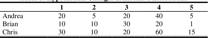
Fields (2000), imagine the following societies numbered from 1 to 5, formed by 3 individuals (these are somewhat extreme examples, but serve to point out the sources of disagreement):

Table 1: Hypothetical Changes in Income Distributions

1 2 3 4 5

Andrea 20 5 20 40 5

Brian 10 10 30 20 1

Chris 30 10 20 60 15

Any relative measure of mobility would indicate that, in going from society 1 to society 2, there has been perfect mobility. The correlation between the two, indeed, is zero. But note that average wealth has gone down and, as a result, so have income levels for all but one of the individuals. The transition from society 2 to society 3, where the correlation is 0.5 – mobility is much lower – but all incomes have gone up, is the mirror image of the first. In this sense, it could be argued that the movement from 2 to 3 is more desirable than from 1 to 2.

The main point here is that relative measures of mobility do not take changes in the average income level into account. While this is seen as a flaw by researchers who would

say that an environment where all incomes are growing is “mobile” or “dynamic”, even if

social ranks are not moving, we believe that mobility concerns arise mainly because of relative considerations. In other words, societies tend to favor situations where

individuals’ relative status is considerably independent from their parents’ degree of

success, and this is best captured by measures of relative mobility.

One distinction should be noted with regard to measures of relative mobility. Positional movement takes place when an individual changes her position in the overall distribution. Related to this is sharemovement, which focuses on the change in an individual’s share of the overall total.2 Both are instances of what Behrman (2000) calls “relative” or

“exchange” mobility.

A process whereby all members double their incomes would be perfectly immobile under both measures (this would correspond to going from society 1 to society 4). Also, a process in which total income decreases and inequality increases while ranks remain the same would show no positional mobility, but shares would have changed (this is the case in going from distribution 4 to 5). Rankings can also change drastically with very little change in income, as is the case in the shift from society 2 to society 5.3

2 _{Although we are trying to avoid referring to “income” in order to drive home the point that we are}

interested in a broader notion of “social” mobility, it is clear that there must be some quantitative element

in order to talk meaningfully about “shares”.

3

The aim is to isolate the distributional component from mobility. We believe that mobility concerns are entirely related to ranks; thus, there may be social mobility even if the overall distribution becomes more unequal. In any case, the lesson to be learned from these examples is that a complete picture of the desirability of an income process cannot be derived from any one summary measure because changes in average income levels, changes in the overall distribution, and the degree to which relative performance in one generation depends on relative performance in the past must all be taken into account.

Absolute movement measures, in contrast, focus on quantifying the total change, regardless of whether any exchange mobility has taken place. We will not go into detailed definitions of these instruments here, however, since they do not seem to be relevant to the type of concern that drives this study.

Although we may be content with quantifying movement – whatever definition we decide upon – it is usually the case that we also want to capture other aspects of movement. In particular, studies of social mobility are generally concerned with gauging how dependent final outcomes are on initial conditions. In other words, income mobility may exist because individual incomes follow an identical random process, independent of initial income, or there may be some sort of dependence – usually captured by a correlation coefficient – between income realizations for the same individual (or dynasty) across time. Most studies of mobility equate time dependence with immobility and, generally speaking, this is the approach that is favored in this paper.

We believe that the concept of mobility is quite distinct from that of economic growth and is closely connected to notions of efficiency, fairness, and political conflict which follow paths that are largely unconnected to overall growth. This is why we choose to focus on measures of relative, rather than absolute, mobility. As will be made clear in this paper, the time span to be chosen will depend on the context of the analysis, while the issue of time dependence will invariably play an important role: increasing social mobility implies breaking the dependence of individual economic outcomes on initial conditions.

Normative Analysis of the Correlation Coefficient

A low correlation coefficient indicates that mobility is high and that parental income is weakly correlated with individual income, whereas a high correlation coefficient signals low mobility. However, authors such as Swift (2005) and Feldman et al. (2000) claim that a zero correlation is not a morally desirable goal because any serious attempt to disconnect the life-income of parents and their offspring would severely compromise important values of family life and privacy. Thus, they argue, instead of pursuing the objective of zero intergenerational correlation, we should ask ourselves which mechanisms of intergenerational transmission are unfair and should then design our

made here is that, just as reporting on inequality does not seem complete without studying mobility,

policies accordingly. Following the same line of reasoning, Jencks and Tach (2005) claim that if we want to know whether opportunity is becoming more or less equal, we need to track intergenerational linkages that violate certain norms associated with meritocracies and developmental opportunity. Under their definition of developmental opportunity, society must either make families and communities more alike or find ways to offset the adverse effect of growing up in a disadvantaged family or community.

Implicit in the reasoning of these authors is the idea that some sources of advantages are acceptable or even desirable while others not. For instance, many people agree that ethnicity should not be a source of advantage, but that effort should. Family contacts, intelligence, or other genetic or environmental traits are more debatable. Therefore, if acceptable sources of advantages are somehow inherited by children of advantaged parents, we would observe a positive correlation between parental and individual incomes even if no unacceptable source of advantages remained.

However, even if all sources of unacceptable advantages were eliminated and the correlation between parental and individual income were fully explained by acceptable advantages, we could still argue that policy interventions to help the disadvantaged would reduce the correlation. Normative evaluation of such policies would ultimately depend on the social preferences of the evaluator and his preference for mobility per se.

Relation with Other Distributional Features

Concerns about static aspects of a society’s welfare distribution – such as inequality, poverty or polarization – are, as a rule, intimately connected with any discussion on social mobility. Most theoretical studies focus on the joint determination of mobility and inequality, since concepts such as poverty and polarization are hard to incorporate into a model. We will therefore examine the relationships between inequality and mobility.

The most common characterization points to inequality as being “a snapshot” of the income-generating process at any point in time, while mobility is seen as tracking income distribution over time based on individual trajectories. When considered from this standpoint, the absence of mobility accentuates all issues associated with inequality. It also underscores the fact that a comparison between the prevailing income distributions in two societies –two “snapshots” – may reverse when mobility is incorporated into the analysis.

This reversal would only happen if higher mobility were somehow associated with higher

inequality and vice versa, so that superficially “equal” societies might actually have more

persistent inequality than highly unequal societies. As we will see, this is far from obvious, and theoretical models as well as empirical evidence provide mixed results. In fact, the most prevalent theoretical association between mobility and inequality is negative, since structural conditions that lead to low mobility also tend to favor unequal outcomes.

Becker and Tomes (1979) were one of the first to model income mobility and inequality. In their economy, there is a continuum of dynasties. Each generation values its own consumption as well as its offspring’s income:





 _{t t t}

t U Z I

U (1)

where Ut is parents’ utility, Ztstands for parents’ consumption, and It+1 is the adult wealth

of their children.

This wealth is embodied in a stock of human and nonhuman capital that has three sources: a direct investment from each generation’s parents (y); endowed “luck” that is correlated across contiguous generations of the same dynasty (e) (which can be interpreted as ability, intelligence, social background or values, and family connections); and sheer market luck (u).

In other words, we think of individuals in this model as helping their children out in two

ways. They can decide to leave them “capital” by investing in their education or

providing them with financial capital. This is a deliberate decision on the part of the

parents. In addition, they pass on family characteristics that were assigned by “luck” to

each dynasty. Parents cannot alter such characteristics or prevent them from being transmitted. A natural interpretation would involve genetic characteristics, but there are

also family connections, “norms” or “customs” within each household, as well as other

non-biological traits, that are largely the result of each family’s history and that cannot be radically changed by any individual dynasty. A poor parent cannot build family connections out of thin air.

Of course, there is a final element of “luck” in determining individual income; people

will typically differ in the extent to which they take full advantage of their endowment, and their resourcefulness or drive may lead them to find new opportunities. Serendipity may also intervene. This is the way in which the term u should be interpreted.

As can be seen from equation (2), each part of this capital stock has the same (constant) market return, w.4 Parents are assumed to be risk-neutral and to choose their bequests in order to maximize their own expected utility, subject to a budget constraint (where r is the intergenerational rate of return),

1 1

1

t t

t t

t

w y

Z I

r

 

 

 (3)

4

Thus, both inequality and mobility refer to the distribution of capital stock or of all sources of income.

1 1 1 1 1 1 1

t t t t t t t

and a law of motion for endowed luck that depends on the family endowment and the average level of endowed luck in the economy.





1 1 1

t t t t

e_   h f e he v_ (4)

In this law of motion, h represents the fraction of family endowment that is inherited, and f is the aggregate rate of growth, while v is a random shock. We thus allow for slow

changes in family “luck”. It may be the case that a rich family loses part of its connections, or that someone from a family that does not value “hard work” may still turn

out to be hardworking and pass this trait on to his children. In any case, as we will see, h is a very important parameter of the model, as it measures the extent to which family

“luck” is equalized across dynasties. When h is close to 0, family endowments are basically identical, with some random variation. When it is close to 1, dynasties differ permanently.

Families fully anticipate inherited endowment (presumably, any relevant “random”

shocks to ability, personality, or the like can be observed before making the optimal investments), but not random luck. From standard expected utility maximization, and normalizing r and w to equal 1, the income of children in the t+1 generation of the ith family can be expressed as:

1 1 1

i i i i i

t t t t t

I_ aI he v_ u_ (5)

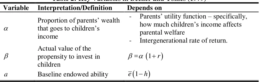
Using Table 2, equation (5) says that income in a given generation basically depends on parental wealth and endowments, although an additional effect is generated through endowed and market luck. Crucially, parental preferences determine how strong this dependence is. This model captures the fact that anticipated luck affects how much capital parents leave to their offspring, which is why both market and endowment luck are not fully appropriated by their children (they only get to enjoy a proportion  ).

Table 2: Key Variables in Becker and Tomes (1979) Variable Interpretation/Definition Depends on

 Proportion of parents’ wealth _{that goes to children’s}

income

- Parents’ utility function – specifically,

how much children’s income affects

parental welfare

- Intergenerational rate of return.

 Actual value of the propensity to invest in children

=





a Baseline endowed ability e











1 1

1 1 1

0 0

1 1

k k

i k i i

t t k t k

k k

a h

I u v

h h  _{  }                     _{ }

 





and the (squared) coefficient of the variation in income – a measure of inequality5– is:













2 1 2 1 1 2

1 1 1

I u e

h

CV CV CV

h           

   (7)

That is, inequality has two components: one that comes from market luck (u), and one that comes from endowed advantages (e).6 Clearly, if any of these components were less variable, income inequality would go down. The additional insight derived from this model comes through the effects of  and h.

Note that the coefficient for endowed family luck is larger than the coefficient for market luck. The difference between them grows as  and h become larger. That is, as we increase the actual value of the propensity of each generation to invest in the next and the degree of family inheritability of characteristics that affect income, we give greater weight in overall inequality to family-specific advantages.

However, whereas an increase in h unambiguously increases inequality, an increase in

 – say, as the result of a change in preferences or through an increase in market returns

– reduces the coefficient of variation in income. This is the result of the fact that, while it increases the variance in income, it increases the level of income even more.

We next turn to income mobility and then analyze how  and h affect the trade-off between inequality and mobility. The preferred measure of income mobility in this article is the effect of an increase in income for generation t on the incomes of subsequent

generations. This gives us an idea of how quickly “temporary” increases in social standing fade away. It measures how long it takes to go “from rags to riches and back”.

In other words, it captures our preferred concept of mobility as the degree of dependence of current outcomes on past performance. Lower persistence is equivalent to higher mobility.

5

The coefficient of variation of a random variable is defined as the ratio of its standard deviation to its mean. That is, CV x

 

by average endowed luck, or e.

6

The last term actually reflects exogenous variation in endowed luck, since

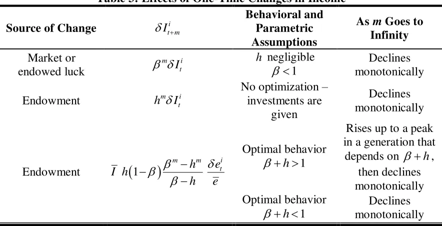
Table 3: Effects of One-Time Changes in Income

Source of Change It mi

Behavioral and Parametric Assumptions

As m Goes to

Infinity Market or endowed luck m i t I

  h negligible

1

  monotonically Declines

Endowment hmIti

No optimization – investments are

given

Declines monotonically

Endowment





i m m t e h I h h e        Optimal behavior 1 h   

Rises up to a peak in a generation that

depends on h, then declines monotonically Optimal behavior

1 h

   monotonically Declines

This effect will depend on the source of the increase in income and, as the authors show, its magnitude hinges on the interplay between optimizing behavior and inheritability. Indeed, if we call I_t a change in income for generation t, and we trace changes in the mth generation, we can envision the different scenarios described in Table 3.

When the degree of inheritability of endowed luck is close to zero, a look at equation 5 tells us that each generation will receive a fraction  of any change in the income of the previous generation, regardless of the source of this income. This change will decrease as the distance between generations increases, given our assumption that 1. In other words, when families do not provide sizeable (dis)advantages to their offspring, mobility is high.

If inheritability was high, but investments were not influenced by changes in endowments

– that is, if families did not optimize – we would see a similar response to a change in endowment. However, if we take into account the fact that families do optimize, we can see that, for some parameter values, a change in family endowment at time t can

compound over time before it fades away (implying that a “lucky” generation will make its descendants luckier than average for a relatively long time). This is exactly the result that we would associate with a lack of social mobility.

This is intuitive: if family connections or race become more important in determining individual income, we would expect differences between families to become more pronounced and permanent.

When the propensity to invest in children goes up, mobility again is reduced, because a one-time shock to income takes more time to fade away. However, in the long run, income differences are reduced, so income inequality goes down.

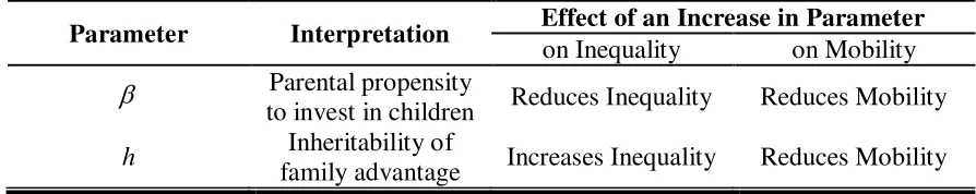
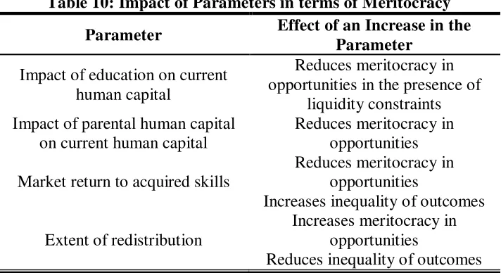
We can summarize these findings in the following table.

Table 4: Relationship between Inequality and Mobility when Parameter Values Change

Parameter Interpretation Effect of an Increase in Parameter on Inequality on Mobility

 Parental propensity

to invest in children Reduces Inequality Reduces Mobility

h Inheritability of

family advantage Increases Inequality Reduces Mobility

Clearly,  is not a parameter that can be manipulated by public policy. It is quite impractical and, arguably, even unethical for the state to try to convince parents to care

less (or more) for their children’s well-being. However, it is not implausible for alterations in h to fall within the scope of public policy. Note that a decrease in h is equivalent to a homogenization of endowments. That is, a decline in h makes endowments more likely to equal the average. Hence, a policy that, for example, calls for investments to be made in raising the quality of public education while making it more homogeneous7 would probably redund in a decrease of h. Note that this reduction would also tend to reduce inequality.

Another way of changing h is by promoting meritocratic employment policies, possibly through encouragement of market competition among potential employers. Why would market competition help attain a meritocracy? Advantages in the labor market that are not related to higher productivity – such as race or family connections – can only persist if companies that engage in these hiring practices are shielded from their consequences. Firms in a competitive environment, in contrast, will come under pressure to adopt practices that favor productivity over personal loyalties or racial prejudice.

The main claim underlying these suggestions is that policies that break the dependence of outcomes on initial conditions are unambiguously desirable.

Becker and Tomes (1979) abstract from the determination of the return to human capital, equating it to physical capital and operating within a stationary economy. Although the basic insight – that mobility and inequality are affected by the way in which parents optimize when making their decisions, as well as by inheritance of personal qualities – is

7

not in dispute, some unbundling of the process of human capital accumulation as an additional force driving inequality and mobility remains to be done. We will comment on two lines of work. One focuses on purely economic forces, while the second adds politico-economic considerations.

Building on Becker and Tomes: Human Capital and Credit Constraints

Hassler, Rodríguez Mora and Zeira (2003) and Owen and Weil (1998) show how inequality and mobility may be jointly determined in a general equilibrium model with overlapping generations of workers. In both cases, they draw a distinction between skilled and unskilled workers. They analyze mobility by determining the odds that the child of an uneducated worker will become skilled (upward mobility), or the odds that the child of a skilled worker will not receive an education (downward mobility).8

The key issue in both models is the lack of access to a credit market, since such access

would allow “high-ability” individuals to invest in their education. This is a very practical concern, inasmuch as it has the consequence of making educational decisions (and, therefore, income) strongly dependent on parental background. In other words, it is a reinterpretation of the parameter h in the Becker and Tomes (1979) model.

Both models assume that ability is not genetically determined. This is why credit market failures end up accounting for most of inefficient immobility. The key point to bear in mind, though, is that this is a simplifying assumption which serves to highlight what aspects other than genetic endowments may affect intergenerational mobility. These effects would persist even if ability were, to some degree, genetically inherited.

Owen and Weil: Liquidity Constraints and Multiple Equilibria

Owen and Weil (1998) model the joint determination of aggregate output, income distribution, mobility, and returns to education in general equilibrium. Skilled and unskilled labors are complements in production, and changes in returns to skill stem from changes in the aggregate supply of each kind of labor.9 In other words, a large supply of unskilled workers increases the skill premium, and vice versa.

Agents differ across two dimensions: they receive different parental transfers, and they are born with different ability levels. Ability is independent across generations and is defined as the amount of efficiency units supplied to the labor market, regardless of skill level (which, instead, affects the wage level at which those units are rewarded). Thus,

ability is not genetically determined and can be likened to “industriousness” (i.e., how

hardworking a person is).

8

Note that these two probabilities may move in opposite directions: a policy that increases overall educational achievement may raise upward mobility and reduce downward mobility. Thus, we once again run into the problem of clearly defining what we want to include in the definition of mobility, or must ask ourselves whether bundling all these phenomena into one concept even makes sense.

9

The timing is as follows. Individuals can be said to live through two stages. In the first, they receive transfers from their parents, then choose an educational level, and work. In the second, they consume and leave a bequest to their children.

An individual can acquire skills by buying education at a fixed cost e. If we call i t

q an

individual’s ability level and s t

w the wage for skill level s, then we find that there is an ability threshold above which it pays to become educated.10 In an efficient outcome, individuals whose ability level exceeds this threshold will obtain an education.

*

t e u

t t

e q

w w



 (8)

However, there are no credit markets available to finance educational decisions. This means that parental bequests (x) are the only source of funding. Thus, individual resources are given by:

*

, , ,

, ,

e i

i t i t t t i t

u i t i t t

x e q w if x e and q q x q w otherwise

   

 (9)

In other words, agents will receive an education only if their bequests enable them to afford it.

Resources are split between individual consumption and bequests to children, with  being the weight that is given by parents to bequests.





  

  

U x_ c_  x_   c_ (10)

Clearly, in choosing a given bequest level, parents are determining the expected value of

their children’s education level. For instance, a bequest lower than e ensures that children will be unskilled workers.

The optimal decisions of each family define, for each distribution of labor supply and each level of wages, what the transfers and resulting education levels will be for the next generation. The authors look for a steady state of this model – a relative wage level and skill distribution such that:

- Families expect wages to stay the same and therefore choose transfers in such a way that the education distribution remains unchanged; and

- Given the education distribution, this wage level is the outcome of market equilibrium.

10

In other words, the starting point for the situation is such that the economy will remain in the same state indefinitely.

Owen and Weil find that when individuals face liquidity constraints, there are multiple steady-state equilibria which exhibit a positive association between equality and mobility. That is, whenever there is high mobility, there is low inequality.

There can, of course, also be a situation in which there is no mobility at all. In such a situation, a handful of skilled workers have high wages that enable them to educate all of their children while wages for unskilled workers are so low that education is not affordable, even for the most industrious families. In fact, when the cost of education is high enough, this is the only kind of steady state there is.11

When the cost of education is below a certain ceiling, there is at least one high-income, high-mobility equilibrium. In such a situation, the workforce is highly educated, which lowers the equilibrium skill wage premium and hence the chances that an unskilled worker will find herself limited by her borrowing constraint. This not only reduces inequality; it also makes it easier for a high-ability child of an unskilled worker to receive an education and lowers the incentive for a low-ability child of a skilled worker to acquire skills. In other words, it raises both upward and downward mobility.

In addition, in these equilibria the allocation of education is more sensitive to actual ability and less so to parental background than it is in a more unequal economy where borrowing constraints are disproportionately greater for the children of low-income parents. This is, in fact, why income is higher, as the most industrious workers are in high-productivity positions.

In low-income societies, these conclusions are reversed: the stock of skills is small, the wage differential is high (so is inequality), and mobility is very low. As a consequence, the allocation of resources is more inefficient.12

Thus, credit market imperfections make current skill levels dependent on past skill levels, as embodied in parental income. The inefficient steady states arise from the fact that this dependence is not based on a productivity difference (as would be the case if, for instance, ability were inheritable).

The key aspect of this model is that these different steady states coexist as possible outcomes for the same economy. In other words, two economies with the same parameters (access to the same technology, equal weight given to children in the utility function) may end up with widely different mobility and inequality levels. If it were possible to change the situation in one period by means of a single (large-scale) policy

11

There can also be a continuum of this sort of immobile steady state. Starting from any one of these states, we can slightly increase the proportion of educated individuals and reduce the wage differential accordingly, and we will have another steady state with no mobility.

12

intervention, it would become self-sustainable. In contrast, the interventions required in economies where it is a question of changing the fundamentals, such as Becker and Tomes, are generally long-term policy measures.

What would a “one-time” intervention involve? One possibility would be a large-scale redistribution of income that could be accomplished either by giving funds directly to parents, by giving them “vouchers” for education, or by using income tax revenues to subsidize public education – anything that would temporarily break the dependence of education on background, thereby increasing the supply of educated workers and moving the system toward a low-inequality, high-income steady state.

Other policy recommendations come from “outside” the model. The focus on human

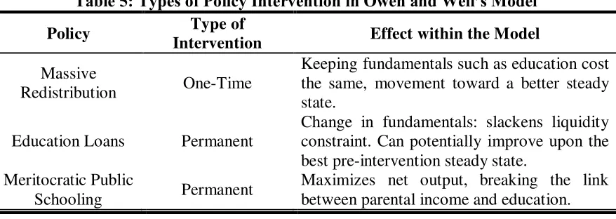
capital acquisition allows Owen and Weil to consider different policy experiments, all of them related to changes in the education system. Given that inefficiencies result from the presence of liquidity constraints, a (permanent) program of education loans is the first option considered. These authors find that such a program reduces inequality and raises average income, effectively moving the economy to a high-education, low-inequality steady state. The second policy they analyze is a meritocratic public education system, where high-ability individuals get the education that maximizes net output. Again, this kind of policy effectively does away with the inefficiencies created by the borrowing constraint. Whether this kind of policy is materially feasible in low-income, low-mobility countries depends on functional forms adopted in the model.13

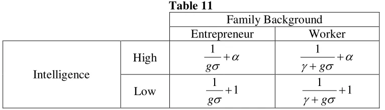
Why would the implementation of a meritocratic schooling system be an effective policy? The answer is that such a system would tend to wipe out the differences in schooling that arise solely by virtue of parental income: in other words, for the same reason that we argued that an increase in schooling quality would reduce h and therefore increase mobility. Note that this is not an abstract consideration. Countries such as China, South Korea and Japan have a strong public education sector which uses testing and assessments early on as a basis for assigning students to schools and channeling them into careers based on their cognitive ability. To a lesser extent, European countries such as Germany and France have a strong, high-quality public education sector as well. These countries also have greater social mobility than Latin America.

Table 5: Types of Policy Intervention in Owen and Weil’s Model

Policy Type of

Intervention Effect within the Model

Massive

Redistribution One-Time

Keeping fundamentals such as education cost the same, movement toward a better steady state.

Education Loans Permanent

Change in fundamentals: slackens liquidity constraint. Can potentially improve upon the best pre-intervention steady state.

Meritocratic Public

Schooling Permanent

Maximizes net output, breaking the link between parental income and education.

13

So far, the effects of differences in background are unambiguously inefficient. However, this changes when skilled parents transmit advantages because they are, in some sense, more efficient than their unskilled counterparts.

Hassler, Rodriguez Mora and Zeira: The Roles of Education and Technology

Moving on, Hassler, Rodriguez Mora and Zeira (2003) present a similar setup in which workers may be skilled or unskilled and must finance their education without access to a loan market. In their setting, however, different agents face different costs of education. In order to become skilled, a child needs a certain amount of schooling time, and this is affected by two factors: innate ability (which is independent across generations and reduces the time needed), and parental background. High-ability individuals need to spend less time obtaining formal schooling in order to acquire skills, and the same is true for children of skilled parents, who need less outside help in order to achieve the same goals, presumably because they have a better understanding of what needs to be done and how best to do it. This is an additional, and plausible, pathway through which parental

background affects children’s well-being.

There are two alternative technologies in this economy: a constant-returns-to-scale production sector, where each skilled worker produces output according to her productivity, and a sector which uses unskilled workers and natural resources as inputs (with such resources being assumed to be equally divided among unskilled workers). The difference between skilled and unskilled workers lies in their productivity, a, which can take two values, a_s a_n, according to the skill level.

s s

n n

y a y a x



 (11)

In an equilibrium, skilled workers will earn a_s, while unskilled workers will earn

n n

X a x a

N



 _  

 

  , where X is the aggregate stock of natural resources and N the aggregate supply of unskilled labor. The income of unskilled workers decreases when the aggregate supply of unskilled workers rises (since 

 

Teachers are hired to provide this schooling time (i.e., to “produce education”) and are paid the skilled-wage rate. Each skilled worker who is employed as a teacher produces a certain amount of units of education: h1. This links innate ability and parental background to education costs: the less outside time needed for the acquisition of skills, the lower the cost of skill acquisition.

consume, and invest in education for their children. They derive utility from their own consumption and from the well-being of their offspring:14

 

par par off

V  c E V (12)

where E is the expectations operator, and V is generational utility.

The process used to model education starts out by specifying innate ability. This is indicated by the amount of time that a person would need to be educated in order to become skilled, if born to a skilled parent. It is labeled inaptitude and denoted by e (and is assumed to be uniformly distributed between 0 and 1). The educational barrier faced by children of unskilled parents is introduced by saying that an individual with inaptitude e needs be units of education in order to become skilled if born to an unskilled household, with b1. Note that when background is introduced in this way, its effect is not

“inefficient,” since it actually requires more resources to educate children from poor families. This differs from the effect of liquidity constraints, which are also present in the model and which limit educational investment even if it would be efficient to invest in an

individual’s education, given her innate ability.

This model has a unique steady state whose equilibrium we will now examine. Under this model, parents will choose to invest in their children’s education if:













ln ln

/

/

s n

s

s

y i V y V

e h y if parent is skilled where i

be h y if parent is unskilled

 

   

 (13)

Because of the structure of preferences, both kinds of parents will choose to spend a maximum fraction of their income in education, which we will call m15. This fraction is chosen optimally, given the value of education (i.e., the difference in expected welfare between skilled and unskilled individuals).

In turn, m defines two threshold inaptitude levels, such that parents will only invest in education for lower values of e. These thresholds satisfy:

s

s s s

n n

s n n

s

e

y my e hm

h

be y hm hm

y my e

h y b Ib

  

    (14)

14

It should be noted that they do not care about the amount of resources spent on their children in and of itself, but rather about the result of their expenditure.

15

Where I is the measure of income inequality chosen by the authors, given by the ratio between the incomes of skilled and unskilled workers:

s

n

y I

y

 (15)

Note that, given the distributional assumptions of e, these thresholds give the probability that the son of a skilled (or unskilled) worker will be skilled and thus serve as indicators of mobility. As expected, the probability that the child of an unskilled worker will become skilled is lower than it is for the son of a skilled worker.

Now, we want to solve for the gains to education as a function of the fraction of income that is spent in equilibrium in order to solve for the optimal m, given the outcomes in the labor market:





n

1

V ln 1 ln 1

s

V I h m m

bI

 _{  }

   _  _{ }   _

  (16)

What does equation (16) tell us? The gains from education are increasing in inequality. This effect is propagated through a direct channel in the form of what could be termed an income effect, but it is also generated by the fact that it increases the likelihood that children from skilled backgrounds will be more able to afford an education than children from unskilled backgrounds. This amplifies the advantage of being born to a skilled parent. We can also see that gains from education rise when the share of income that is allotted to education increases.

In order to close the model, we need to know the share of individuals who will be unskilled in equilibrium, which will in turn determine relative wages. In other words, we need to take into account what happens in the labor market. For every ratio of skilled to unskilled labor supply, there is a corresponding inequality level, which in turn influences the proportion of income that goes into education. In a steady state, this ratio will be such that the optimal education demands generated will keep the proportions of skilled and unskilled unchanged in the following generation.

Since the model defines a unique steady-state equilibrium, comparative statics come from changes in the model parameters. The key finding is that there is no unique correlation between inequality and upward mobility (measured by the probability that an individual born to an unskilled family will become skilled, e_n). As we have previously shown, this level is given by e_n hM I

 

Ib

 , where we have incorporated the fact that the share of

income going into education is endogenous.

There are two effects. Through M I

 

effect, which is created by the difficulty of paying for a teacher when the wage differential is high. This is the distance effect. At low levels of inequality, the incentive effect dominates. When inequality is high, the distance effect prevails.

Table 6: Effects of an Increase in Inequality When Initial Inequality is

Low High

Higher Inequality Increases Mobility Reduces Mobility

Of course, inequality is endogenous and depends on the labor market’s structural

conditions. Hence, Hassler, Rodriguez Mora and Zeira first analyze exogenous changes in the production sector. Skill-biased technical change raises the wage differential for any given workforce skill composition. This kind of change increases the incentive to acquire education, thereby raising the proportion of income that goes into education. It also increases inequality, and this latter effect acquires greater weight when inequality is already high. In other words, skill-biased technical change increases inequality the most in economies which were already unequal. The change in mobility mirrors what we said above: for low levels of initial inequality, skill-biased technical change increases upward mobility; for high levels of inequality, it reduces mobility.

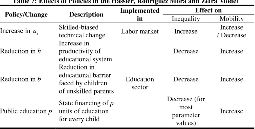
The second set of exogenous changes that these authors analyze relates to the educational sector, that is, changes in h and b. An increase in h, i.e., in the overall productivity of education, has two general equilibrium effects: it increases upward mobility, and it reduces inequality. A reduction in the educational barrier faced by children from unskilled backgrounds, as measured by b, has a less clear effect. By making investment by unskilled parents more productive, it reduces the fraction of income invested in education across the board. This implies greater downward mobility, as children from high-skill backgrounds become more likely to forgo an education. However, it can still be shown that inequality goes down as mobility goes up.

Table 7: Effects of Policies in the Hassler, Rodriguez Mora and Zeira Model

Policy/Change Description Implemented in

Effect on

Inequality Mobility

Increase in a_s Skilled-biased

technical change Labor market Increase

Increase / Decrease

Reduction in h

Increase in productivity of educational system

Education sector

Decrease Increase

Reduction in b

Reduction in educational barrier faced by children of unskilled parents

Decrease Increase

Public education p

State financing of p units of education for every child

Decrease (for most parameter

values)

The last change that is analyzed is the introduction of public education, which amounts to a certain level of education, p, being purchased by the government (financed by taxes) and given to all children, with parents being free to supplement that education with additional outlays. These authors further assume that there is a proportional tax on income, T, and that h equals 1. With these additions to the original model, the education thresholds are modified and turn into:









1 1

s n

m

e p m T e p T

b I

 

    _   _

  (17)

The main point is that skilled parents make more effective use of public education. Carrying out a general equilibrium analysis similar to the one used in the original model, including the relationship between taxes and the level of public education, the authors conclude that an increase in public education raises upward mobility and, unless both  and b are too close to 1, reduces inequality.

Summarizing the findings in Table 7, we see that, here again, public interventions that operate through the educational sector tend to induce a virtuous cycle of reduced inequality and increased mobility. However, it is possible that higher inequality will be met by higher mobility, particularly when the factors driving the increases come from the labor market and are the result of changes in technology.

Although these three models emphasize different aspects of the determination of income inequality and intergenerational mobility, they share a number of common aspects. The main intuition is that the more parental background determines individual outcomes, the more likely it is that high inequality will be associated with lower mobility. In Becker and Tomes (1979), reducing the degree of inheritability lowers inequality and raises mobility, which is effectively the same as reducing the educational barriers faced by children of unskilled parents in the Hassler, Rodríguez Mora and Zeira (HMZ) (2003) model or relaxing the tightness of the borrowing constraint in the Owen and Weil (1998) model. In contrast, when we increase incentives to invest in children starting from a relatively equal setup, we may find that inequality increases together with mobility. This is what happens in the Becker and Tomes model, as well as in the HMZ setup, when skill-biased technical change increases the incentive to education.

These models both suggest a natural constraint on how much mobility can be changed and point to policies that may affect it. If ability is intrinsically inheritable, as is the family endowment in the Becker and Tomes model, then it is a source of permanent differences between dynasties and a brake on social mobility. However, this also suggests

that efforts to “level the playing field” through the use of such measures as compulsory

3. INEQUALITY AND MOBILITY: POLITICO-ECONOMIC CONSIDERATIONS

So far, we have abstracted from the actual workings of governments. A vast amount of literature discusses how politico-economic considerations affect the distribution of income, as well as social mobility, when considered intertemporally. We will now discuss these kinds of results.

At this point, we are mainly interested in the association between inequality and mobility, rather than in the politico-economic consequences of mobility per se (which we deal with in a separate section). The main findings discussed in the literature are summarized in Benabou (1996).

This author sets up an overlapping generations model in which generations within a dynasty are not altruistic toward each other. The utility of each generation is given by:

ln ln

i i i

t t t

U  c  d (18)

where c is consumption when young and d is consumption when old. People are endowed with resources w distributed independently and identically across dynasties. These resources can be invested in capital and used to generate second-period income, according to the technology used:

   

i i

t t t

y r k  w  (19)

where k is the amount of the investment and wt is the average level of resources in the

community. Given that there are imperfect capital markets, k is limited by individual resources – that is, k_ti w_ti.

The linkage between generations comes through this resource level, which can be interpreted as the endowment of basic skills: skills possessed by young agents are derived

from the interaction between parents’ incomes as adults – determined by their own skill level – and innate ability, which is independent across generations. Thus:

1 1

i i i

t t t

w_ _ y (20)

There is a political element in the model which comes in the form of income taxation and redistribution before individual investment decisions are made. For convenience, the author adopts a log-linear specification, whereby post-redistribution income is given by:

 

 

ˆi i

t t t

y  y  y  (21)

where yt is determined by budget balance. The tax scheme is progressive when 





process. In order to incorporate the possibility of systems or societies with different levels of wealth bias, Benabou introduces the variable p, which indicates the position in the wealth distribution of the pivotal voter. Higher p implies higher wealth bias.

When a system displays a pro-poor bias, in the sense that the pivotal voter is poorer than the mean, the economy converges toward a unique steady state. The stronger the populist bias, the higher redistribution and mobility are and the lower after-tax inequality is. Thus, we see an inverse relation between inequality and mobility, as greater equality is associated with higher mobility, which in this case is induced by political considerations.

When a system exhibits a pro-rich bias, however, multiple steady states are possible. Equilibria with low redistribution have high (after-tax) inequality and lower mobility. They are also less efficient than equilibria with higher redistribution. Thus, we again find that inequality and mobility are inversely correlated. Both are jointly determined by the nature of the political system, which in turn affects the cross-sectional wealth distribution, and by the degree to which it persists from generation to generation.

4. SOCIAL MOBILITY, EQUALITY OF OPPORTUNITY AND

MERITOCRACY

A sizeable portion of the literature on social mobility links it with both equality of opportunity and meritocracy, but without – for the most part – specifying the precise conceptual link between these notions.16 In some cases, these two concepts are taken to be almost exact synonyms, while in others they are considered to be related ideas that sometimes have a causal link. This ambiguity is attributable partly to a certain disregard for semantic discussions by the economic community and partly to the intrinsic difficulty

of defining “equality of opportunity” and “meritocracy”. In the next sections, we will

attempt to shed some light on these concepts.

Equal Opportunity and Social Mobility

Numerous authors have given a nuanced treatment to the definition of equality of opportunity and its relationship to notions of fairness and justice.17 We do not attempt to provide a full survey, but rather simply a definition that draws on different sources and is intuitively appealing.

16

In fact, Benabou and Ok (2001b) argue that since equal opportunity is usually seen as the reason why mobility is desirable, the degree of mobility in the income process should be ranked according to how strongly opportunities are equalized.

17

As we mentioned in the discussion on mobility, in every society there are certain generally desirable social outcomes with regard to income, status, and the like. Egalitarian philosophies of justice suggest that some sort of equality should prevail in the distribution of these outcomes. Equality in the opportunity to achieve these goals, as opposed to equality in the actual distribution of outcomes, seems to reflect the most widespread view of what constitutes a fair situation. It is what the “equal playing field” metaphor refers to, and it seems to have almost universal appeal.18

What exactly, then, is equality of opportunity? Drawing from the common elements in Dworkin (1981), Roemer (1998, 2004) and Sen (2000), we can sketch out a very simple

model that helps illustrate this concept. Say that an individual’s outcomes depend on her

effort and her circumstances. Effort relates to all actions willfully undertaken by the individual that potentially affect her attainment of the desired outcome. Circumstances, on the other hand, refer to aspects of the environment that affect the likelihood of

attaining the goal but that are largely beyond the individual’s power to change. In a

society which values equality of opportunity, individuals will be held responsible for differences in outcomes stemming from differential effort, but not for those that result from two agents applying the same effort level starting from different circumstances.

This brief description highlights the common element and the sources of diverging opinions among proponents of equality of opportunity. As for the common element, note that equality of outcomes per se is not deemed desirable a priori. Instead, differences in effort (chosen autonomously by each individual) make differential outcomes not only acceptable, but desirable. Differences arise, though, when the time comes to decide what

constitutes “circumstance” and what constitutes “effort” and, hence, in determining how

far the equalization of outcomes should go.

One extreme view is to define “equal opportunity” as “non-discrimination”. Under this definition, guaranteeing that people are judged by their qualifications only – for instance, when applying for a job – is enough to achieve equal opportunity. In this case, the

relevant circumstances are taken to be “irrelevant” factors that are generally beyond the individual’s ability to change: gender, or race, or other such characteristics. If, on the

other hand, only college-educated individuals are given a chance to compete for a given job, this is not considered to be unfair. The implicit assumption is that everyone has had the opportunity to acquire the relevant skills and that those who did not do so should be accountable for their choice.

The opposite extreme is represented by egalitarians such as, for instance, John Roemer (1998), who departs from this view in two significant ways. First, he argues that the set of relevant circumstances should include innate ability, family background (in terms of connections and of attitudes toward effort, availability of role models, and the like), peer group effects, and all factors that affect individual preferences but that come into play before an individual can be reasonably expected to notice their importance. To make the

18

This is the theme of the 2005 World Development Report (World Bank, 2005); a large proportion of

point explicit, he would argue that whether an individual was raised in an affluent suburb where parents expect their children to go to college or whether he was born into a poor family where scholastic performance was not deemed important are factors that should be regarded as individual circumstances.

The second departure is that he proposes that effort should not be quantified independently from circumstances. That is, he argues that the effort expended by an individual who completes a two-year post-secondary degree despite having been raised in an environment where the median educational level is that of a high school dropout is greater than the effort made by a college graduate who comes from a well-to-do setting in which the median educational achievement is the completion of a college degree. In effect, he suggests circumstances should be used to define groups that serve as a benchmark for gauging individual effort. He also calls for a broad definition of what

factors actually constitute “circumstances”.19

Most opinions lie somewhere in the wide expanse existing between these extremes. Most people would accept the proposition that family connections and privileges should not matter in determining lifetime income and status. Possibly fewer would agree with the idea that differences in innate cognitive or physical ability should play a significant role.20 It is fair to say that relatively few would want to compensate individuals for differences in their preferences that lead them to exert less effort than similar individuals, regardless of where those preferences come from.

At this point, we should see a clear difference between meritocracy and equality of

opportunity as we have defined it here, although we may want to count as “merits”

aspects that are effectively circumstances. For instance, we may find it plausible that the work ethic of immigrant children is not really of their own doing, yet still believe it is morally defensible to reward them for their deeds. This underscores the fact that equality of opportunity may have the wide support it enjoys partly because of the looseness with which the concept is usually employed.

We will now explore the connection between equal opportunity and social mobility. Both terms are frequently used interchangeably, yet our previous discussion should have established the fact that perfect mobility will only be equivalent to perfect equality of opportunity if we adopt an extreme view of what circumstances should be compensated for when equalizing opportunity.

By our preferred measures, perfect social mobility implies no correlation between parental and offspring outcomes. How could this come about in an actual economic

19

Roemer (1998) goes as far as to argue that for the children of Asian immigrants in the US, median educational achievement is higher because of their heritage, which encourages them to excel at school; thus, they should not enjoy a higher status as adults than children from African-American families who were equally poor and unconnected to begin with, but whose environment made it unimportant to go to school.

20