Visualization of 3-dimensional bargaining problems

Visualization of 3-dimensional

bargaining problems

Laura S´

anchez

, Silvia Castro

, Luis Quintas

_{Dpto. Inform´atica y Estad´ıstica, UNC, Neuqu´en, Argentina}

[email protected]

(2)

_{Dpto. Cs.de la Computaci´on, UNS, Bah´ıa Blanca, Argentina}

[email protected]

(3)

_{Dpto.Matem´atica, UNSL, San Luis, Argentina}

[email protected]

Abstract

This paper presents a visualization in three dimensions of the classical solutions of thebargaining problem for 3 agents. It provides a helpful tool for game theorists, economists and other researchers and professionals in these areas in order to visualize and compare the solutions over a wide family of bargaining problems and gain intuition about general results.

The theory of bargaining, a branch of the Cooperative Game Theory, tries to find reasonable solutions when two or more agents have to decide over a wide variety of possible agreements among a family of conflictive situations.

1

Introduction

The theory of bargaining, a branch of the Cooperative Game Theory, tries to find reasonable solutions when two or more agents have to decide over a wide variety of possible agreements among a family of conflictive situations. The basis of Bargain-ing Theory can be found in the paper by Nash ([Nash 50]). He developed a formal model of the following situation: Two agents having a feasible set of alternatives can agree on a particular one. In this case, this one will be the solution to the bargaining problem; otherwise, they end up at a prespecified feasible alternative representing the disagreement (disagreement point). Nash developed a theory attempting to pre-dict how the agents should establish a compromise of their preferences over a family of conflictive situations. He analyzed a restricted natural class of bargaining prob-lems and formulated axioms which solutions should satisfy. He also established the existence of a unique solution that satisfies all the axioms. In this way, Nash estab-lished the bases of the axiomatic theory of bargaining. His solution was regarded as

the solution until the seventies, when other solutions were introduced. Since then there has been many activities in this field and numerous solutions have been pro-posed in the literature. There are a lot of parameters entering in the description of the problem and it is not easy to compare and analize the behavior of different solutions for the different situations without an automatic tool.

First we give the theoretical background for the bargaining theory. Then we de-scribe briefly the work made on bargaining problem visualization until now. After that, we detaile the motivation for our work and give an overview of the implemen-tation of the visualization. Finally, we give the conclusions and some directions on future work.

2

Theoretical Background

2.1

Domains

We consider now the fundamental points on the theoretical formulation of the bar-gaining problem. Ann−agent Bargainig Problem, is a pair (S, d) whereSis a subset of the n−dimensional Euclidean space (ℜn_{) and d is a point of S. Let} Pn

d be the

class of problems such that

- S is convex, bounded and closed (contains its boundary) - d∈S being d a strictly dominant point

- It exist p∈S with p > d

(1)

agreement. Given p, p′ _{∈ ℜ}n_{, p≥p}′ _{means p}

i ≥p′i for all i and p6=p′ ; the relation

p > p′ _{means p}

i > p′i for all i.

S is the feasible set, i.e. each point p ∈ S is a feasible alternative and the coordinates of p give the utility profits (measured in von Neumann - Morgenstern utilities) for each one of the n agents. dis the disagreement point. Additionally, we said that a pair (S, d) ∈ Pn

d is d−comprehensive if p ∈ S and p ≥ q ≥ d implies

that q∈S.

We usually work with a normalized domain where the disagreement point is the origin of coordinates and some additional restrictions are imposed on the domains. The bargaining problems are then restricted to the class of problems Pn

0, i.e. the

subclass of Pn

d consisting of the pairs (S, d) such that they fulfill the conditions

given in (1) and also the following:

-d= 0 -S ⊆ ℜn

+

- ifp∈S then any q ∈ ℜn _{with 0≤q≤p is also inS (ie, q ∈S)}

(2)

If these three conditions (2) are also satisfied we say that S is 0−comprehensive, or just comprehensive. In summary, we usually deal with the subclass (Pn

0) of

problems S, that constitutes an important class for economic applications.

2.2

Solutions

Given a bargaining problem, a solution is a function from the domain to a particular point in the domain and represents the agreement reached by the agents.

We formally state that asolution is a functionF :Pn

→ ℜn_{such thatF(S, d)∈}

S (see [Thompson 94]).

The boundary BS of S, could be defined as:

BS ={p∈S |∄ p′ _{∈S with p}′ _{> p}}

Then, the solution associates with each element (S, d) of the domain an unique point ofS interpreted as a recommendation for that problem, and that point will be on the boundary, also defined like theconvex and comprehensive convex hull (CCH).

2.3

Typical Solutions

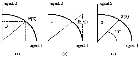
Three solutions play a central role in the theory as it appears today. The first one was theNash Solution. Nash gave a list of axioms that characterized his solution (see [Thompson 94]) and tried to capture some properties of fairness and optimality. In the case ofP2

dhis solution,N(S, d), is obtained maximizing the area of the rectangle

Besides the fact that the Nash solution seemed to be very reasonable for most bargaining problems, in some cases it did not take into account the aspirations of the agents (see [Thompson 94]) It was in the 70 ’s whenKalai-Smorodinsky ([Kalai 75]) proposed an alternative solution (KS(N, d)). It chooses the most preferred feasible alternative in the line going from the origin of coordinates to the point consisting of the maximum aspiration of each agent (Fig 1(b)). This is perhaps the second more accepted solution.

The third solution, theEgalitarian,E(S, d), ([Thompson 94]) gives the maximum equal utility alternative to each agent (Fig. 1(c)). This idea of equal gains is central to many theories of social choice and welfare economics.

Thompson presents in his comprehensive survey ([Thompson 94]) other typical solutions. There are also other class of solutions favoring one agent at the expense of the others, but much work should be done to extend this solutions when the number of agents is greater than 2.

Figure 1: Typical solutions to the bargaining problem (a) Nash (b) Kalai-Smorodinsky (c) Egalitarian

3

Related Work

Besides the analytical studies mentioned above, there is very few said about how solutions perform over different sets of Bargaining Problems. This is a very inter-esting problem, but at the same time very difficult. It is not easy to foresee general properties, but if we hope to be successful in finding those properties, it would be helpful to have a tool for solving a wide set of problems. With this aim Cavalie, Quintas and Welch ([Cavalie 97]) provided a computational tool for 2-agents bar-gaining problems. It was helpful in providing a wide family of barbar-gaining problems and also has proved to be a very useful tool for teaching.

4

Extension to 3D

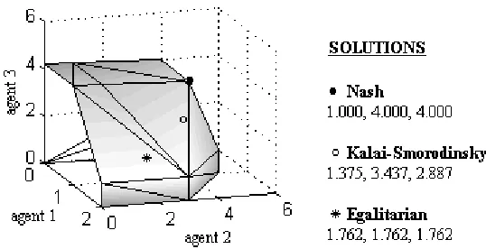
will be usually a point in the 3D Comprehensive Convex Hull (CCH) of a certain set (Fig. 2). In this case we can model the interaction of three agents for different sets of (S, d) pairs. This certainly enriches the discussion on the solutions, giving an extra complexity to the analysis, and allowing an approach to a larger set of real situations.

Figure 2: Example

There is very few written in the literature for the three dimensional case. This tool has proved to be very useful one in order to visualize diferent sets of (S, d) pairs. It is also a must in order to gain intuition about general properties. We can just mention some discussions on the different ways of extending some classical solution to this case (see [Thompson 94]), that we have also implemented.

4.1

Comprehensive Convex Hull Representation and

Gen-eration

The feasible set for the three dimensional case (three agents) will be represented by the volume enclosed by the comprehensive convex hull (CCH). This CCH, that represents the space where the three agents could obtain optimal profits, will be represented by a triangulated surface denoted by SF or shell of a set of points, in the positive octant of the three dimensional space.

4.1.1 Data Structure

decomposition, i.e. a triangulation. The surface SF could be described without ambiguities like a collection of three primitive elements and their mutual adjacency relationships. The primitive elements are:

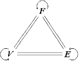
• Vertices (V) • Edges (E) • Faces (F)

From the nine pairwise ordered adjacency relations (Fig. 3), that can be defined over the three primitive topological elements, the Symmetric Data Structure (see [Woo 85]), encodes the three primitive elements of a 3D triangulation and four of their mutual adjacency relations representing the topology without ambiguities.

Figure 3: The nine pairwise ordered adjacency relations

We use the Modified Symmetric Data Structure (see [de Floriani 87]) to built and manipulate the triangulation. This structure encodes the three basic elements of the triangulation plus three constant (relationsF E,EV andEF) and one partial relations (relationV E∗_{). It is showed in (see [de Floriani 87]) that such a structure} is optimal (up to a constant factor) with respect to both space and time complexity. The time complexity is evaluated in terms of the worst case complexity of those structure accessing algorithm, which retrieve partial relations, i.e. relations that are not stored in the data structure.

For each primitive element of the triangulation T, this data structure encodes the following relations:

• For each face f, a list of index to the sourrounding edges, in counterclockwise order:

RelationF E

F E(f) = [e1, e2, e3], f ∈ F. F is the set of faces of T and [e1, e2, e3], the

• For each edge e, indexes to the extreme points of e and to the two incident faces. In this case, the stored relations are:

RelationEV

EV(e) = [v1, v2], e∈E. E is the set of edges ofT and [v1, v2] the ordered pair

of vertices ofT, which are extremes of edge e. RelationEF

EF(e) = [f1, f2], e ∈ E. E is the set of edges of T and [f1, f2] the sequence

of faces of T sharing the edge e. Following the edge orientation, f1 is the left

face and f2 the rigth face of e.

• For each vertex, the geometry and an index to one of the incident edges on that vertex

Partial relation V E∗

V E∗_{(v) ={e}

i},v ∈V. V is the set of vertices ofT and {ei}is one edge of T,

incident onv.

The topology of the triangulation is then represented without ambiguities with the three primitive elements (F, E, V) and the subset of the four adjacency rela-tions. This subset of relations, gives a topological description of the triangulation

T and assures the eficiency of the algorithms that access the data structure (see [Weiler 85],[Woo 85]).

4.1.2 Modified Convex Hull in 3D (CCH)

In order to generate our shell, we obtain the surfaceSF like a comprehensive convex hull,CCH of 3Dpoints. TheCCH is stored in a symmetric modified data structure detailed in the previous section. We calculate theCCHk using an incremental

algo-rithm, that allows a point to be added interactively without completely recalculate the shell. The addition of a point to a convex hull, is based in the algorithm given in ([de Berg 97]). The shell is in the positive octant and limited by the planes x = 0,

y= 0 and z = 0. Given a pointp, the shell CCHk will be calculated as follows:

A set must be created with all the projections of p on each coordinated plane and on each coordinated positive axis.

• If k = 0, the CCH does not exist, and the initial shell must be created with

p and all its projections.

• If k >0, the CCH is the shell of k points and we have two different cases:

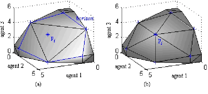
2. Ifpis exterior to the shellCCHk, we construct a set of points to be added

to theCCHk with p and all the projected pointspi that are exteriors to

the CCH_k. In order to do that, we look from p_i to the shell in the direction of the coordinated origin. From this point, some faces or all can be seen. These faces are the visible region of pi and are limited by a

closed curve: thehorizon ofp_i in theCCH_k+i−1 (Fig. 4(a)). This horizon

is the boundary between the visible and the invisible faces. The visible ones must be eliminated and replaced by the faces connecting pi and its

horizon (Fig. 4(b)).

Figure 4: Addition of a pointpi to the comprehensive convex hull (CCH)

The CCH is stored in a symmetric modified data structure detailed in the pre-vious section.

Algorithm Shell

IN: CCHk being

k= 0 if the CCH does not exist

k >0 if CCH is a shell of k points

pbeing the point to be incorporated to the CCHk

OUT:CCHk′being  



k′ _{=k if pis interior or belongs to the input shell}

k′ _=k+n if p and then−1 points that generatesp are incorporated to the CCHk

Generate all the projections of pon each plane x= 0, y= 0 and z = 0, and also on each axis x,y and z, i.e.

Proj ← {px=0, py=0, p z=0, px axis, py axis, p z axis}

If CCHk is empty

then

Generate CCH with p and all the projections: Proj ←Proj∪ {p}

IncorporatePoints(Proj, CCHk)

if p is not interior and do not belongs to theCCHk

for each pi ∈Proj

if p_i is interior or belongs to the CCH_k

then

Proj ←Proj− {pi}

Proj ←Proj∪ {p}

IncorporatePoints(Proj, CCHk)

Algorithm IncorporatePoints

IN: CCHk being

k= 0 if the CCH do not exist

k >0 if CCH is a shell of k points

Proj being the set of points to be incorporated to the CCHk

OUT:CCHk′being k′ =k+n wheren is the amount of points stored in Proj

for each pi ∈Proj

{insert p_i inCCH_k+i−1}

VisFaces ← visibles faces from pi

Horizont ← List of edges forming the horizont of VisFaces Eliminate VisFaces of CCHk+i−1

for each edge∈ Horizont

Connect edge topi creating a triangular face

Add the face the CCHk+i−1

5

Conclusions and Future Work

There is very few written in the literature about the three dimensional case. The visualization we have presented has proved to be very useful for the visualization of different sets of bargaining problems and their solutions for 3−agents. Before this tool, it was very difficult to visualize different experimental sets because it is very tedious to obtain them and its solutions manually.

We hope that this visualization we have developed will also be very useful in order to gain insight about general properties for the solutions to the bargaining problems in the three dimensional case, as happened in the 2-dimensional case.

As future work we propose

• From the theoretical point of view, to extend the 2-dimensional solutions to the 3D case. In this situation, the extension of this visualization envisions to be of great help.

We also plan to use all these visualizations integrated in a visualization tool for teaching the courses including topics in Bargaining Theory.

6

Bibliography

References

[Cavalie 97] Cavali´e, P., Welch, D., Quintas, L., ”Implementaci´on Computa-cional a las soluciones cl´asicas del problema del regateo”, Proceed-ings COMDEX/INFOCOM’97, Bs. As., Argentina, 199-212, 1997.

[de Berg 97] de Berg, M., van Kreveld, M., Overmars, M., Schwarzkopf, O., ”Computational Geometry ”, Springer Verlag, 1997.

[de Floriani 87] de Floriani, L., ”Surface Representation based on triangular grids

”, The Visual Computer, 3(1):27-50.

[Nash 50] Nash, J. F., ”The Bargaining Problem”, Econometrica, 28:155-162, 1950.

[Kalai 75] Kalai, E. , M. Smorodinsky, ”Others Solutions to Nash’s Bargaining Problem”, Econometrica, 43:513-518, 1975.

[Thompson 94] Thompson, W., ”Cooperative Models of Bargaining”, Handbook of Game Theory with economic applications, vol 2, North Holland, 1994.

[Weiler 85] Weiler, K. ”Edge-based data structures for solid modeling in curved-surface environments ”, IEEE Computer Graphics and Applica-tions, 5(1):21-40, January 1985.