Abstract—This paper presents results about power system stabilizers (PSS) coordination in multi-machine power systems. Due to their versatility, power system stabilizers have been employed extensively to enhance the power oscillations damping. One of the main tasks within this context is to estimate the best PSS’s parameters. In this paper, this is solved by a neural network. The applicability of the proposal is demonstrated by simulation on two test systems. Results show that the proposed stabilizers’ coordination is comparable to that obtained by a conventional design, without requiring a detailed model analysis.
Index Terms—Multimachine grid, power system stabilizer, simultaneous tuning, stability.
I. INTRODUCTION
variety of controllers have been developed to enhance the power oscillations damping. Important efforts are made to achieve their best performance.
A practical PSS must be robust over a wide range of operating conditions and capable of damping the oscillating modes. From this perspective, the conventional single input PSS design approach based on a single machine infinite bus (SMIB) linearized model exhibits some deficiencies: (i) There are uncertainties in the linearized model resulting from the variation in the operating condition, since the linearization coefficients are derived typically under nominal operating conditions.
(ii) Various techniques like PID, artificial neural network, GA-fuzzy, hybrid neuro-fuzzy, adaptive fuzzy logic, simulated annealing, pole-shifting, etc., have been tested to achieve tuning under various operating conditions for the single input PSS. However, the single input PSS may lack robustness in a multi-machine power system.
In a power system stabilizer, the electrical power and the rotor angular speed variation ∆ω are calculated from the generator’s voltage and current values. In stationary operation, deviations in the electrical power are used to evaluate the optimum stabilizing signal in terms of the amplitude and phase relationship by means of a lead/lag filter.
Manuscript received May 25, 2011; revised May 25, 2011. This work was supported in part by the FOMIX-CONACyT Hidalgo under grant 130107 and CFE-CONACyT under grant 88160.
Ruben Tapia, Omar Aguilar, Felipe Coyotl are with the Engineering Department, Universidad Politécnica de Tulancingo, Calle Ingenierías 100, Huapalcalco, Hidalgo, México.(phone: 775-755-8202; fax: 775-755-8321; e-mail: rtapia,[oaguilar],[fcoyotl]@upt.edu.mx).
Juan Manuel Ramirez is with the Electrical Engineering Department, CINVESTAV, Av. del Bosque 1145, colonia el Bajío, Zapopan, 45019, Jalisco, México. (e-mail: [email protected]).
Currently, power stations employ conventional PSSs with lead-lag structure. Over the last two decades, various PSS parameters’ tuning schemes have been developed and applied to solve the problem of electromechanical modes damping. Modern control techniques have been proposed to coordinate the stabilizers [1-8].
The PSS parameters’ tuning has been approached by two major strategies, sequential tuning and simultaneous tuning. In order to obtain the set of optimal PSS parameters under various operating conditions, the tuning and testing of PSS parameters must be repeated under various operating conditions. Therefore, if the sequential tuning method is applied to tune the PSS parameters, the parameters tuning will become more intricate. On the other hand, in the case that the simultaneous tuning method is employed to tune the PSS parameters, which can simultaneously relocate and coordinate the eigenvalues for various oscillating modes under different operating conditions, the long computation time could be a drawback in large power systems.
The adaptive PSS concept may be categorized into two research approaches: direct and passive. Direct tuning refers to adaptively changing PSS parameters online and thus achieving higher controllability of inter-area oscillations [9]. In contrary, passive design focuses on optimizing the observability of the PSS by adaptively varying the strength of the input signals. Although both approaches can enhance the stability of inter-area mode, passive designs have not been widely explored. The motivation of this paper is to investigate the possibility of updating on-line the PSS gains to enhance the damping of inter-area oscillations. This is to ensure that minimal modifications are done to the existing infrastructure. The objective is to adaptively adjust the gains in accordance to the present grid operating condition. This is achieved by a strategy to update conventional PSSs currently operating in power systems that were tuned time ago. The main idea is to re-tune basically the PSS’s gains through an on-line procedure, which involve a few measurements. After that, the same stabilizers may continue working properly under different operating conditions and topologies. Results show that this idea works adequately, independently of the studied power system.
II. MODELING A. Power system model
In this paper, two power systems available in the open research are employed in order to exemplify the proposition. The development of systematic methodologies for PSS tuning is a problem that requires special attention. Once it is determined that a system requires effective damping, especially for the electromechanical modes, the fundamental problem is to find the best control parameters (static or
Simultaneous Coordination for PSS Parameters
Ruben Tapia, Juan Manuel Ramirez, Omar Aguilar, and Felipe Coyotl
dynamic). The deficiency of damping can be solved by means of power systems stabilizers. However, it is necessary to apply a coordination algorithm. In this paper, an on-line strategy is applied to re-tune PSSs in order to adapt them to new conditions.
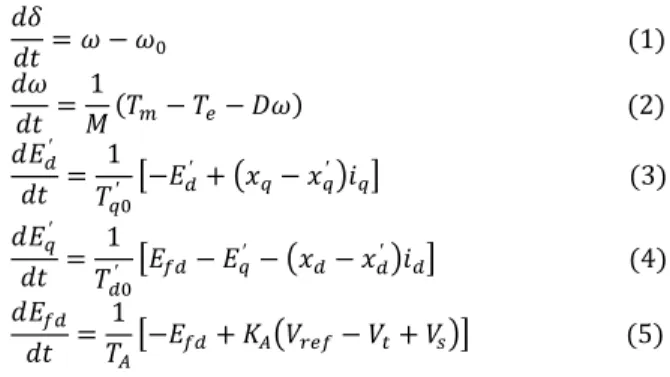
The fourth order dynamic model is utilized for generators including a static excitation system [10]. The set of equations for each generator becomes:
= − (1)
= (1 − − ) (2)
′
= 1
′ −
′ +
− ′ (3)
′
=1′ −
′ −
− ′ (4)
= 1
−+ ! "#− "$+ "% (5)
where (rad) and (rad/s) represent the rotor angular position and angular velocity; ′ (pu) and ′ (pu) are the internal transient voltages of the synchronous generator; (pu) is the excitation voltage; (pu) and (pu) are the d- and q-axis currents; ′ (s) and ′ (s) are the d- and
q-open-circuit transient time constants; ′ (pu) and
′ (pu) are the d- and q- transient reactances; (pu) and (pu) are the d- and q- synchronous reactances; (pu) and (pu) are the mechanical and electromagnetic nominal torque; is the inertia constant; is the damping factor; ! and (s) are the system excitation gain and time constant; "# is the voltage reference; "$ is the terminal voltage magnitude; "% is the PSS’s output signal.
B. PSS model
The interaction between stabilizers may increase or decrease the damping of certain oscillating rotor modes. To have a better performance, a proper coordination of all control devices used in the network is required, while also ensuring the robustness under different operating conditions. A typical static excitation system has "% as input, (5), which is the PSS’s output. The structure of a conventional PSS connected to the k-th machine consists of a gain, a washout unit, units of phase compensation, and an output limiter, Fig. 1. The washout unit is used to prevent state changes of the input signal by changing the terminal voltage. In this paper, both parameters, the gain ' and the time constant , are updated on-line to attain a proper performance under different operating conditions, without restructuring this control in a power station. In order to illustrate the procedure, it is assumed the use of the angular velocity deviation, (), as the PSS’s input, Fig. 1.
Fig. 1. PSS block diagram.
To simplify the procedure, it is assumed that += , and
-= .. These parameters remain in their original values. Of course, these ones could be updated too.
III. PROPOSITION
The major advantages of the artificial neural networks (ANNs) are the controller’s design simplicity, and their compromise between the complexity of a conventional nonlinear controller and its performance. The B-spline neural networks (B-SNNs) are a particular case of neural networks that allow to control and model systems adaptively, with the option of carrying out such tasks on-line, and taking into account the power grid non-linearities. A B-spline function is a piecewise polynomial mapping, which is formed from a linear combination of basis functions, and the multivariate basis functions are defined on a lattice [11].
Through B-SNN there is the possibility to bound the input space by the basis functions definition. Generally, only a fixed number of basis functions participate in the network’s output. Therefore, not all the weights have to be calculated each sample time, thus reducing the computational effort and time.
The B-SNN’s output can be described by [11],
/ = 012 (6)
w
[
]
Tp
w w
w K
2 1
= , a
[
]
Tp
a a
a K
2 1
=
where 4) and 5) are the i-th weight and the i-th B-SNN basis function output, respectively; p is the number of weighting factors.
In this paper it is proposed that ' and be updated through one B-spline neural network, respectively, Fig. 1. The angular velocity deviation from its nominal value, ey, is
the input signal to adapt the gain '. While the generator’s active power deviation from its nominal capacity, ez, is the
input signal to adapt the time constant . Such election is made based on the close relationship between active power and velocity respect to the damping, (2). Then the network can be described as follows:
' = 66)78, 4) (7)
= 66)(7:, 4)) (8)
where i denotes the B-spline network which is used to
update ' and ; wi is the corresponding weighting factor;
= 1,2, …pss number. Fig. 2 depicts a scheme of the proposed B-spline neural network. It is noteworthy that this block will substitute the wash-out block in Fig. 1, in order to introduce an adaptive strategy.
Fig. 2. B-SNN to update the PSS gains.
sT sT k
+
1 2
1 1 1
sT sT
+ +
4 3
1 1
sT sT + + ( )s
U Vs( )s
sT sT k
+
1 2
1 1 1
sT sT
+ +
4 3
1 1
sT sT + + ( )s
Ui Vs( )s
ω ∆
max _
s
V
min _
s
V
sT sT k
+
1 2
1 1 1
sT sT
+ +
4 3
1 1
sT sT + + ( )s
U Vs( )s
sT sT k
+
1 2
1 1 1
sT sT
+ +
4 3
1 1
sT sT + + ( )s
Ui Vs( )s
ω ∆
sT sT k
+
1 2
1 1 1
sT sT
+ +
4 3
1 1
sT sT + + ( )s
U Vs( )s
sT sT k
+
1 2
1 1 1
sT sT
+ +
4 3
1 1
sT sT + + ( )s
Ui Vs( )s
ω ∆
max _
s
V
min _
s
V
P G
k
output
1
a
) (t ez
weight vector basis
f unctions input
1
The appropriate design requires the following a-priori information: the bounded values of ey and ez, the size, shape,
and overlap definition of the basis function. Such information allows to bound the B-SNN input and to enhance the convergence and stability of the instantaneous adaptive rule [11]. Likewise, with this information the B-SNN estimates the optimal weights’ value. The neural networks controllers, (7)-(8), are created by univariate basis functions of order 3, considering that both ey and ez are
bounded within [-1.0, 1.0] pu.
A. Learning
Learning in ANN is usually achieved by minimizing the network’s error, which is a measure of its performance, and is defined as the difference between the actual output vector of the network and the desired one.
On-line learning of continuous functions, mostly via gradient based methods on a differentiable error measure is one of the most powerful and commonly used approaches to train large layered networks in general [12], and for non-stationary tasks in particular.
In this application, the parameters’ quick updating is looked for. While conventional adaptive techniques are suitable to represent objects with slowly changing parameters, they can hardly handle complex systems with multiple operating modes. The instantaneous training rules provide an alternative so that the weights are continually updated and reach the convergence to the optimal values. Also, conventional nets sometimes do not converge, or their training takes too much time [12-14].
In this paper, the ANN is trained on-line using the following error-correction instantaneous learning rule [11],
4)() = 4)( − 1) +>0()>=7)()
--5)() (9)
whereη is the learning rate and 7)() is the instantaneous output error.
Respect to the learning rate, it takes as initial value one point within the interval [0, 2] due to stability purposes [11]. This value is adjusted by trial-and-error. If η is set close to 0, the training becomes slow. On the contrary, if this value is large, oscillations may occur. In this application, it settles down in 0.0057 for ', and 0.00136 for .
It is proposed that during the actualization procedure, a dead band is included to improve the learning rule convergence. The weighting factors are not updated if the error has a value below 5%,
4)() = @4)( − 1) +
=7)()
>a()>--5)(), if|7)| > 0.03
4)( − 1), otherwise
F (10)
This learning rule has been elected as an alternative to those that use, for instance, Newton’s algorithms for updating the weights [13-14] that require Hessian and Jacobian matrix evaluation. (9) has been obtained through the minimization of the output’s mean square error, using descendent gradient rules. That is the reason because it is said that the weights converge to optimal values [11].
Thus, the proposition consists fundamentally on
establishing its structure (the definition of the basis functions) and the value of the learning rate. Regarding the weights’ updating, (9) should be applied for each input-output pair in each sample time; the updating occurs if the error is different from zero. Respect to the learning rate, it takes as initial point one value inside the interval [0, 2] due to stability purposes [11]. This value is adjusted through trial-and-error; with a value close to zero the training becomes slow. Hence, the B-SNN training process is carry out continuously on-line, while the weights’ value are updated using only two feedback variables.
IV. TEST RESULTS AND ANALYSIS
In order to demonstrate that this proposition has feasibility, two multimachine power systems of the open research are employed. The proposed tuning performance is exhibited. To analyze the results, simulations are developed under different scenarios: (i) with PSS tuned by optimization [15] (static parameters), FXPSS; (ii) with PSS tuned by B-SNN (dynamic parameters), ANNPSS. Several operating conditions are taken into account.
A. Case 1
In this section the 39-bus, 10-generator test system is analyzed [16]. To examine the results four conditions are presented. Comparisons are made with the response obtained using a PSS with fixed parameters, Fig. 3-6; the PSSs data is summarized in the Appendix.
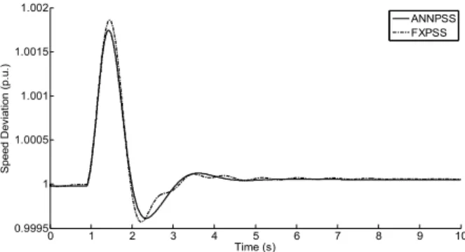
The first condition shows the system’s evolution when it is subjected to a three-phase fault at bus-38 with duration of 95-ms; after that time the fault is cleared. Fig. 3 displays the evolution of the speed deviation in generator 2. Quite similar results are exhibited.
Fig. 3. Angular velocity in generator-2, condition 1.
The second condition illustrates the system evolution under a three-phase fault in bus-31, lasting for 85ms; after that, the fault is cleared without reconfiguration. Fig. 4 shows that the dynamic behavior of the proposed scheme is better than that of the conventional PSS with fixed parameters.
The third case validates the appropriate system evolution under a three-phase fault at bus-28, lasting for 85-ms; after that time, the fault is cleared by tripping line 26-28. The performance of the tuning technique is in accordance with conditions 1 and 2. The ANNPSS exhibits very well performance adapting itself to the new conditions, Fig. 5.
0 1 2 3 4 5 6 7 8 9 10
0.9995 1 1.0005 1.001 1.0015 1.002
Time (s)
S
p
e
e
d
D
e
v
ia
ti
o
n
(
p
.u
.)
Fig. 4. Reactive power in generator-4, condition 2.
Fig. 5. Angular difference δ5-1 considering machine 1 as reference,
condition 3.
The following condition displays the system evolution when the generator’s active power is increased 9 percent, while the loads are increased 9 percent. After that, = 10 s, the system experiences a three-phase fault in bus-24, cleared without reconfiguration. The response of the neural controller has better transient response.
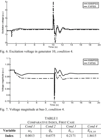
Fig. 6 presents the excitation voltage behavior in generator 10. It is noticed that the transient and steady state response exhibit differences between both controllers. The variation can be understood considering (5), where the PSS signal is injected. Thereby, they can increase or decrease the oscillations and steady state error, depending on their parameters. Furthermore, the dynamic and static excitation voltage behavior has other implication into the system’s variables, such as the terminal voltage. If the PSS parameters are inappropriate, the controller can cause degradation in the generators voltage magnitude and, possibly a decrease in the network nodal voltages. At generator 3 the pre-contingency voltage magnitude 1.0046 pu. After the perturbation, its value is 0.9753 pu with ANNPSS, and 0.9382 pu with FXPSS, which implies a difference of 2.91% and 6.6%, respectively, Fig. 7.
To quantify the difference between two signals, we use the following measure,
GH= IJ KLMM− K)N-
1O$P
$P
(11)
where G is the index; Q = 1,2,3, … variable number; is the analysis time. KLMM is a signal obtained by the proposed procedure. K)N is the same signal, achieved by the conventional PSS with fixed parameters.
This expression is employed to calculate a quantitative index to indicate the disparity between both signals. If there is no variation between the signals mj becomes zero, while
the signals are more different this index is bigger. Table I
presents the bigger index in the previous conditions.
Fig. 6. Excitation voltage in generator 10, condition 4.
Fig. 7. Voltage magnitude at bus-3, condition 4.
TABLEI
COMPARATIVE INDEX,FIRST CASE
Cond 1 Cond 2 Cond 3 Cond 4
Variable - R. S_+ _+
Index 0.0013 0.6575 0.2171 1.8615
B. Second case
The system under test is the New England power system consisting in 16-generators and 68-buses [17]. The proposed strategy allows achieving a satisfactory coordination among the PSSs installed in generators 1-12, and 14-16. The reference generator is that in bus 13 (generator 13), Fig. 8. Four conditions are evaluated:
(i) Three-phase fault at bus-34 without reconfiguration. (ii) In = 0.9 s a three-phase fault at bus-29 is simulated lasting for 85ms. Then, in = 8 s, a three-phase fault at bus-60 is applied. 90 s after the fault is cleared.
(iii) In = 0.9 s a three-phase fault at bus-46 is simulated lasting for 86 ms, followed by tripping line 46-49.
(iv) In = 0.9 s the generator’s active power, excluding generator-13, which is the slack bus, is increased 12 percent, while the loads are increased 12 percent, both reactive and active power. Then, in = 8 s, the system experiences a three-phase fault at bus-43.
Figs. 9-12 depict the system behavior, where satisfactory coordinated performance can be appreciated. Fig. 9 presents the active power evolution in generator-1 under condition 1. The PSSs data is given in the Appendix.
Fig. 10 shows that using the proposed updating, the power system exhibits softer transient, in comparison to the use of conventional PSSs. The ANNPSS has the ability to be updated to a new operating condition, improving the system performance. Fig. 11 exhibits the neural network performance to update the stabilizers parameters, it illustrates the updating procedure. Remaining signals have similar behavior under each contingency.
0 1 2 3 4 5 6 7 8 9
1 1.5 2 2.5 3 3.5
Time (s)
R
e
a
c
ti
v
e
p
o
w
e
r
(p
.u
.)
ANNPSS FXPSS
0 1 2 3 4 5 6 7 8 9
-0.3 -0.28 -0.26 -0.24 -0.22 -0.2 -0.18
Time (s)
A
n
g
u
la
r
d
if
fe
re
n
c
e
(p
.u
.)
ANNPSS FXPSS
0 2 4 6 8 10 12 14 16 18 20
0 1 2 3 4 5
Time (s)
E
x
c
it
a
ti
o
n
v
o
lt
a
g
e
(
p
.u
.)
ANNPSS FXPSS
0 2 4 6 8 10 12 14 16 18 20
0.75 0.8 0.85 0.9 0.95 1 1.05 1.1
Time (s)
V
o
lt
a
g
e
m
a
g
n
it
u
d
e
(
p
.u
.)
Fig. 8. 16-generators and 68-buses power system.
Fig. 9. Active power in generator-1, Case 2, condition 1.
As shown in Fig’s. 9-12 the adaptive controller parameters performance can decrease the oscillations amplitude and transient time under different operating conditions, respect to the behavior with fixed control parameters. Fig. 12 depicts the angular difference of generator 5 respect to the slack. It is noteworthy that under a load increment, the neural controller response is slower than its counterpart with fixed parameters. However, under a three-phase fault at bus-43 the adaptive parameters allow the controller to exhibit quite well performance, while the FXPSS exhibits longer oscillations. Table II present the bigger index, (11), on the previous conditions. This example is clear for concluding that the tuning scheme has better performance for some operation conditions, thus guarantying the satisfactory electric net operation under different conditions.
Table III illustrates the steady-state parameters reached by the neural network, showing that they are updated under different operating conditions. Thus, depending on the power system topology, these parameters modify their value.
TABLEII BIGGER INDEXES,SECOND CASE
Cond 1 Cond 2 Cond 3 Cond 4
Variable + . + _+, S_+, Index 1.0218 0.0045 0.5260 1.1474
Fig. 10. Angular velocity of generator-4, Case 2, condition 2.
Fig. 11. Time constants evolution in generator 11 and 13, Case 2, condition
3.
Fig. 12. Angular difference of generator 5 considering machine-13 as reference, Case 2, condition 4.
N39 10
9 8
1
13 16
15
12
2
6 11
4 5
7 3
N41
N40 N48 N47
N53 N54 N1
N55
N8 N25
N26 N27
N28 N29 N9 N17
N18
N68 N24 N67
N66 N19
N21 N22
N6 N23
N7 N20
N4 N5
N56
N57 N60
N64 N58
N65 N63
N62 N3 N2
N59 N13 N37 N43 N44 N45
N12 N36 N61 N30 N32
N11
N33 N34
N35
N51 N50 N16
N52 N42
N15 N49
N38 N46
N31 N10 14
N14
0 1 2 3 4 5 6
0 1 2 3 4 5 6
Time (s)
A
c
ti
v
e
p
o
w
e
r
(p
.u
.)
ANNPSS FXPSS
0 2 4 6 8 10 12 14 16
0.998 0.999 1 1.001 1.002 1.003
Time (s)
S
p
e
e
d
D
e
v
ia
ti
o
n
(
p
.u
.)
ANNPSS FXPSS
0 1 2 3 4 5 6 7 8 9
7.44 7.46 7.48 7.5 7.52 7.54
Time (s)
T
im
e
c
o
n
s
ta
n
t
(T
)
T
G11
T
G13
0 2 4 6 8 10 12 14 16 18
-0.6 -0.5 -0.4 -0.3 -0.2 -0.1 0 0.1 0.2
Time (s)
A
n
g
u
la
r
d
if
fe
re
n
c
e
(p
.u
.)
TABLEIII
PSSADAPTIVE PARAMETERS IN STEADY STATE
Parameters Cond 1 After fault
34-bus
Cond 2 Cond 3
After fault
46-bus
Cond 4 After fault 43 bus After
fault 29-bus
After fault 60-bus
'
495.3486 35.6189 261.6139 288.2834 304.0524 536.2815 764.5362 211.1964 381.5372 103.2673 627.5677 103.9179 441.0833 847.9418 351.9842
611.0226 282.7528 848.2500 685.0289 304.0524 73.1612 208.8702 410.1681 717.9996 314.3699 141.3750 819.0843 717.9229 847.9418 351.9842
610.9814 679.3898 95.1925 684.9578 474.2157 73.1398 208.7903 410.1218 717.9635 723.6045 118.1730 727.9283 717.9072 847.9418 351.9842
621.5071 282.7528 848.2500 288.2834 304.0524 282.7981 764.5362 763.1140 381.5372 89.2947 373.8036 819.0843 844.0823 847.9418 351.9842
155.8997 226.0278 353.2842 172.9600 633.3205 146.1670 169.5348 763.1140 170.8420 326.8654 233.4197 692.6240 322.7501 138.6969 678.7408
7.4996 7.4998 7.5003 7.5020 7.5015 7.5024 7.5018 7.5010 7.5020 7.5001 7.4994 7.4966 7.5015 7.5035 7.5071
7.5000 7.4998 7.5018 7.4995 7.4999 7.5001 7.4998 7.5001 7.5004 7.4999 7.4986 7.5003 7.5060 7.5061 7.5058
7.5005 7.5020 7.5034 7.4996 7.4997 7.5011 7.5004 7.5012 7.5005 7.5003 7.5009 7.5027 7.5178 7.5143 7.5113
7.5017 7.4991 7.4982 7.4977 7.4982 7.4987 7.4991 7.4989 7.4977 7.5020 7.5001 7.5006 7.5229 7.5281 7.5261
7.4737 7.4787 7.4759 7.4791 7.4963 7.4741 7.4835 7.4965 7.4714 7.4800 7.4738 7.4487 6.9568 6.9883 7.0893
+= , 0.08 0.08 0.08 0.08
-= . 0.015 0.015 0.015 0.015
V. CONCLUSION
The aim of the paper is to show the performance of adaptive PSSs parameters as a mean to enhance power system oscillations. In order to attain such purposes a B-spline Neural Network-based is proposed. With this neural adaptive scheme, the possibility to implement the on-line updating parameters is potential due to it has learning ability and adaptability, robustness, simple algorithm and fast calculations, and not exclusive but inclusive, nature to get better solution under hardware’s constraints. This is desirable for practical hardware implementation in power stations.
Unlike the conventional technique, the B-spline NN exhibits an adaptive behavior since the weights can be adapted on-line responding to inputs and error values as they arise. Also, it can take into account nonlinearities, un-modeled dynamics, and un-measurable noise. Simulations on two multi-machine power systems under different disturbances and operating conditions, demonstrate the effectiveness and robustness of the proposed strategy.
APPENDIX
PSS data 39-bus, 10-generator test system:
' = [435; 197; 593; 202; 212; 197; 535; 534; 267; 220];
= 7.5; += ,= 0.080; -= .= 0.0150, the time constants have the same value for all machines.
PSS data 68-bus, 16-generator test system:
' = [372; 169; 508; 172; 182; 169; 458; 457; 228; 188; 85; 491; 506; 508; 211]; = 7.5; += ,= 0.080;
-= .= 0.0150, the time constants have the same value for all machines.
ACKNOWLEDGMENT
Ruben Tapia, Omar A. and Felipe C., thank FOMIX-CONACyT by support under grant 130107.
Juan M. Ramirez thanks CFE-CONACyT under grant 88160.
REFERENCES
[1] A. L. B. Do Bomfim, G. N. Taranto and D. M. Falcao, “Simultaneous Tuning of Power System Damping Controllers Using Genetic Algorithm,” IEEE Trans. Power Systems, vol. 15, pp. 163-169, February 2000.
[2] Y. L. Abdel -Magic, M. A. Abido, S. Al -Baiyat and A. H. Mantawy, “Simultaneous Stabilization of Multimachine Power Systems Via Genetic Algorithms,” IEEE Trans. Power Systems, vol. 14, pp. 1428-1437, November, 1999.
[3] Y. L. Abdel -Magic, M. A. Abido, and A. H. Mantawy, “Robust Tuning of Power System Stabilizer in Multimachine Power Systems,”
IEEE Trans. Power Systems, vol. 15, pp. 735-740, May. 2000.
[4] M. A. Abido, and Y. L. Abdel -Magic, “Hybridizing Rule -Based Power System Stabilizers with Genetic Algorithms,” IEEE Trans. Power Systems, vol. 14, pp. 600-607, May, 1999.
[5] S.P. Ghoshal, A. Chatterjee, V. Mukherjee, “Bio-inspired fuzzy logic based tuning of power system stabilize,” Expert Systems with
Applications 36 (2009) 9281–9292.
[6] A.M. El-Zonkoly, A.A. Khalil, N.M. Ahmied, “Optimal tunning of lead-lag and fuzzy logic power system stabilizers using particle swarm optimization,” Expert Systems with Applications 36 (2009) 2097–2106.
[7] K. Sebaaa, M. Boudourb, “Optimal locations and tuning of robust power system stabilizer using genetic algorithms.” Electric Power
Systems Research 79 (2009) 406–416.
[8] Sheng-Kuan Wang, Ji-PyngChiou, Chih-Wen Liu, “Parameters tuning of power system stabilizers using improved ant direction hybrid differential evolution,” Electrical Power and Energy Systems 31 (2009) 34–42.
[9] J. C.-H Peng, N. K. C. Nair, A. L. Maryani, and A. Ahmad, “Adaptive Power System Stabilizer Tuning Technique for Damping Inter-Area Oscillations.” IEEE PES General Meeting 2010, Minneapolis, MN., July 2010.
[10] P. M. Anderson and A. A. Fouad, “Power System Control and Stability,” IEEE Press, 2d ed., 2003.
[11] Brown, and C. Harris, “eurofuzzy Adaptive Modelling and Control,” Prentice Hall International, 1994.
[12] David Saad, “On-line learning in neural networks,” Cambridge University Press 1998.
[13] A. H. Osman, Tamer Abdelazim, and O. P. Malik, “Transmission Line Distance Relaying Using” IEEE Transactions on Power Delivery, vol. 20, April 2005, pp. 1257-1264.
[14] A. Osman, T. Abdelazim, and O. P. Malik, “Adaptive distance relaying technique using on-line trained neural network,” in Proc.
IEEE PES General Meeting, Toronto, ON, Canada, Jul. 2003.
[15] Isidro Castillo T., Juan M. Ramírez and R. Tapia, “A Genetic Algorithm Applied to Enhance the Damping of Multi-machine Power Systems,” orth American Power Symposium, College Station, Texas, USA, pp. 618-625, 2001.
[16] K. R. Padiyar, “Power System Dynamics: Stability & Control”, John Wiley and Sons (Asia), 1996.