Strengthening the Reporting of Observational Studies in Epidemiology
(STROBE): Explanation and Elaboration
Jan P. Vandenbroucke, MD; Erik von Elm, MD; Douglas G. Altman, DSc; Peter C. Gøtzsche, MD; Cynthia D. Mulrow, MD; Stuart J. Pocock, PhD; Charles Poole, ScD; James J. Schlesselman, PhD; and Matthias Egger, MD, for the STROBE initiative
Much medical research is observational. The reporting of observa-tional studies is often of insufficient quality. Poor reporting hampers the assessment of the strengths and weaknesses of a study and the generalizability of its results. Taking into account empirical evidence and theoretical considerations, a group of methodologists, research-ers, and editors developed the Strengthening the Reporting of Observational Studies in Epidemiology (STROBE) recommendations to improve the quality of reporting of observational studies.
The STROBE Statement consists of a checklist of 22 items, which relate to the title, abstract, introduction, methods, results, and dis-cussion sections of articles. Eighteen items are common to cohort studies, case– control studies, and cross-sectional studies, and 4 are specific to each of the 3 study designs. The STROBE Statement provides guidance to authors about how to improve the reporting of observational studies and facilitates critical appraisal and
inter-pretation of studies by reviewers, journal editors, and readers. This explanatory and elaboration document is intended to en-hance the use, understanding, and dissemination of the STROBE Statement. The meaning and rationale for each checklist item are presented. For each item, 1 or several published examples and, where possible, references to relevant empirical studies and meth-odological literature are provided. Examples of useful flow diagrams are also included. The STROBE Statement, this document, and the associated Web site (www.strobe-statement.org) should be helpful resources to improve reporting of observational research.
Ann Intern Med.2007;147:W-163–W-194. www.annals.org
For author affiliations, see end of text.
Editor’s Note: In order to encourage dissemination of the STROBE Statement, this article is being published simulta-neously inAnnals of Internal Medicine,Epidemiology, and PLoS Medicine. It is freely accessible on theAnnals of Inter-nal Medicine Web site (www.annals.org) and will also be published on the Web sites ofEpidemiologyandPLoS Med-icine. The authors jointly hold the copyright of this article. For details on further use, see the STROBE Web site (www.strobe -statement.org).
R
ational health care practices require knowledge about the etiology and pathogenesis, diagnosis, prognosis, and treatment of diseases. Randomized trials provide valu-able evidence about treatments and other interventions. However, much of clinical or public health knowledge comes from observational research (1). About 9 of 10 re-search papers published in clinical specialty journals de-scribe observational research (2, 3).THE
STROBE STATEMENT
Reporting of observational research is often not de-tailed and clear enough to assess the strengths and weak-nesses of the investigation (4, 5). To improve the reporting of observational research, we developed a checklist of items that should be addressed: the Strengthening the Reporting of Observational Studies in Epidemiology (STROBE) Statement (Appendix Table). Items relate to the title, ab-stract, introduction, methods, results, and discussion sec-tions of articles. The STROBE Statement has recently been published in several journals (6). Our aim is to ensure clear presentation of what was planned, done, and found in an observational study. We stress that the recommenda-tions are not prescriprecommenda-tions for setting up or conducting
studies, nor do they dictate methodology or mandate a uniform presentation.
STROBE provides general reporting recommenda-tions for descriptive observational studies and studies that investigate associations between exposures and health out-comes. STROBE addresses the 3 main types of observa-tional studies: cohort, case– control, and cross-secobserva-tional studies. Authors use diverse terminology to describe these study designs. For instance, “follow-up study” and “longi-tudinal study” are used as synonyms for “cohort study,” and “prevalence study” as a synonym for “cross-sectional study.” We chose the present terminology because it is in common use. Unfortunately, terminology is often used in-correctly (7) or imprecisely (8). InBox 1, we describe the hallmarks of the 3 study designs.
THE
SCOPE OF
OBSERVATIONAL
RESEARCH
Observational studies serve a wide range of purposes, from reporting a first hint of a potential cause of a disease to verifying the magnitude of previously reported associa-tions. Ideas for studies may arise from clinical observations or from biological insight. Ideas may also arise from infor-mal looks at data that lead to further explorations. Like a clinician who has seen thousands of patients and notes 1 that strikes her attention, the researcher may note some-thing special in the data. Adjusting for multiple looks at
See also:
Appendix Table. The Strengthening the Reporting of Observational Studies in Epidemiology (STROBE) Statement: Checklist of Items That Should Be Addressed in Reports of Observational Studies
Item Item
Number
Recommendation
Title and abstract 1 (a) Indicate the study’s design with a commonly used term in the title or the abstract.
(b) Provide in the abstract an informative and balanced summary of what was done and what was found. Introduction
Background/ rationale
2 Explain the scientific background and rationale for the investigation being reported.
Objectives 3 State specific objectives, including any prespecified hypotheses. Methods
Study design 4 Present key elements of study design early in the paper.
Setting 5 Describe the setting, locations, and relevant dates, including periods of recruitment, exposure, follow-up, and data collection.
Participants 6 (a)Cohort study:Give the eligibility criteria, and the sources and methods of selection of participants. Describe methods of follow-up.
Case–control study:Give the eligibility criteria, and the sources and methods of case ascertainment and control selection. Give the rationale for the choice of cases and controls.
Cross-sectional study:Give the eligibility criteria, and the sources and methods of selection of participants. (b)Cohort study:For matched studies, give matching criteria and number of exposed and unexposed.
Case–control study:For matched studies, give matching criteria and the number of controls per case.
Variables 7 Clearly define all outcomes, exposures, predictors, potential confounders, and effect modifiers. Give diagnostic criteria, if applicable.
Data sources/ measurement
8* For each variable of interest, give sources of data and details of methods of assessment (measurement). Describe comparability of assessment methods if there is more than one group.
Bias 9 Describe any efforts to address potential sources of bias. Study size 10 Explain how the study size was arrived at.
Quantitative variables
11 Explain how quantitative variables were handled in the analyses. If applicable, describe which groupings were chosen, and why.
Statistical methods
12 (a) Describe all statistical methods, including those used to control for confounding. (b) Describe any methods used to examine subgroups and interactions.
(c) Explain how missing data were addressed.
(d)Cohort study:If applicable, explain how loss to follow-up was addressed.
Case–control study:If applicable, explain how matching of cases and controls was addressed.
Cross-sectional study:If applicable, describe analytical methods taking account of sampling strategy. (e) Describe any sensitivity analyses.
Results
Participants 13* (a) Report the numbers of individuals at each stage of the study—e.g., numbers potentially eligible, examined for eligibility, confirmed eligible, included in the study, completing follow-up, and analyzed.
(b) Give reasons for nonparticipation at each stage. (c) Consider use of a flow diagram.
Descriptive data 14* (a) Give characteristics of study participants (e.g., demographic, clinical, social) and information on exposures and potential confounders.
(b) Indicate the number of participants with missing data for each variable of interest. (c)Cohort study:Summarize follow-up time—e.g., average and total amount. Outcome data 15* Cohort study:Report numbers of outcome events or summary measures over time.
Case–control study:Report numbers in each exposure category or summary measures of exposure.
Cross-sectional study:Report numbers of outcome events or summary measures.
Main results 16 (a) Give unadjusted estimates and, if applicable, confounder-adjusted estimates and their precision (e.g., 95% confidence intervals). Make clear which confounders were adjusted for and why they were included. (b) Report category boundaries when continuous variables were categorized.
(c) If relevant, consider translating estimates of relative risk into absolute risk for a meaningful time period. Other analyses 17 Report other analyses done—e.g., analyses of subgroups and interactions and sensitivity analyses.
Discussion
Key results 18 Summarize key results with reference to study objectives.
Limitations 19 Discuss limitations of the study, taking into account sources of potential bias or imprecision. Discuss both direction and magnitude of any potential bias.
Interpretation 20 Give a cautious overall interpretation of results considering objectives, limitations, multiplicity of analyses, results from similar studies, and other relevant evidence.
Generalizability 21 Discuss the generalizability (external validity) of the study results. Other information
Funding 22 Give the source of funding and the role of the funders for the present study and, if applicable, for the original study on which the present article is based.
the data may not be possible or desirable (9), but further studies to confirm or refute initial observations are often needed (10). Existing data may be used to examine new ideas about potential causal factors, and may be sufficient for rejection or confirmation. In other instances, studies follow that are specifically designed to overcome potential problems with previous reports. The latter studies will gather new data and will be planned for that purpose, in contrast to analyses of existing data. This leads to diverse viewpoints, for example, on the merits of looking at sub-groups or the importance of a predetermined sample size. STROBE tries to accommodate these diverse uses of ob-servational research—from discovery to refutation or con-firmation. Where necessary, we will indicate in what cir-cumstances specific recommendations apply.
HOW TO
USE THIS
PAPER
This paper is linked to the shorter STROBE paper that introduced the items of the checklist in several
jour-nals (6), and forms an integral part of the STROBE State-ment. Our intention is to explain how to report research well, not how research should be done. We offer a detailed explanation for each checklist item. Each explanation is preceded by an example of what we consider transparent reporting. This does not mean that the study from which the example was taken was uniformly well reported or well done; nor does it mean that its findings were reliable, in the sense that they were later confirmed by others: It only means that this particular item was well reported in that study. In addition to explanations and examples, we in-cluded boxes with supplementary information. These are intended for readers who want to refresh their memories about some theoretical points or be quickly informed about technical background details. A full understanding of these points may require studying the textbooks or methodological papers that are cited.
topics, such as genetic linkage studies, infectious disease modeling, or case reports and case series (11, 12). As many of the key elements in STROBE apply to these designs, authors who report such studies may nevertheless find our recommendations useful. For authors of observational studies that specifically address diagnostic tests, tumor markers, and genetic associations, STARD (13), REMARK (14), and STREGA (15) recommendations may be partic-ularly useful.
THE
ITEMS IN THE
STROBE CHECKLIST
We now discuss and explain the 22 items in the STROBE checklist (Appendix Table) and give published examples for each item. Some examples have been edited by removing citations or spelling out abbreviations. Eigh-teen items apply to all 3 study designs, whereas 4 are de-sign-specific. Starred items (for example, item 8*) indicate that the information should be given separately for cases and controls in case– control studies, or exposed and unex-posed groups in cohort and cross-sectional studies. We ad-vise authors to address all items somewhere in their paper, but we do not prescribe a precise location or order. For instance, we discuss the reporting of results under a num-ber of separate items, while recognizing that authors might address several items within a single section of text or in a table.
Title and Abstract
1(a) Indicate the study’s design with a commonly used term in the title or the abstract.
Example
“Leukaemia incidence among workers in the shoe and boot manufacturing industry: a case– control study” (18).
Explanation
Readers should be able to easily identify the design that was used from the title or abstract. An explicit, com-monly used term for the study design also helps ensure correct indexing of articles in electronic databases (19, 20).
1(b) Provide in the abstract an informative and balanced summary of what was done and what was found.
Example
“Background: The expected survival of HIV-infected patients is of major public health interest.
Objective: To estimate survival time and age-specific mortality rates of an HIV-infected population compared with that of the general population.
Design: Population-based cohort study.
Setting: All HIV-infected persons receiving care in Denmark from 1995 to 2005.
Patients: Each member of the nationwide Danish HIV Cohort Study was matched with as many as 99 persons
from the general population according to sex, date of birth, and municipality of residence.
Measurements: The authors computed Kaplan–Meier life tables with age as the time scale to estimate survival from age 25 years. Patients with HIV infection and corre-sponding persons from the general population were ob-served from the date of the patient’s HIV diagnosis until death, emigration, or 1 May 2005.
Results: 3990 HIV-infected patients and 379 872 per-sons from the general population were included in the study, yielding 22 744 (median, 5.8 y/person) and 2 689 287 (median, 8.4 y/person) person-years of observa-tion. Three percent of participants were lost to follow-up. From age 25 years, the median survival was 19.9 years (95% CI, 18.5 to 21.3) among patients with HIV infec-tion and 51.1 years (CI, 50.9 to 51.5) among the general population. For HIV-infected patients, survival increased to 32.5 years (CI, 29.4 to 34.7) during the 2000 to 2005 period. In the subgroup that excluded persons with known hepatitis C coinfection (16%), median survival was 38.9 years (CI, 35.4 to 40.1) during this same period. The rel-ative mortality rates for patients with HIV infection com-pared with those for the general population decreased with increasing age, whereas the excess mortality rate increased with increasing age.
Limitations: The observed mortality rates are assumed to apply beyond the current maximum observation time of 10 years.
Conclusions: The estimated median survival is more than 35 years for a young person diagnosed with HIV infection in the late highly active antiretroviral therapy era. However, an ongoing effort is still needed to further reduce mortality rates for these persons compared with the general population” (21).
Explanation
The abstract provides key information that enables readers to understand a study and decide whether to read the article. Typical components include a statement of the research question, a short description of methods and re-sults, and a conclusion (22). Abstracts should summarize key details of studies and should only present information that is provided in the article. We advise presenting key results in a numerical form that includes numbers of par-ticipants, estimates of associations, and appropriate mea-sures of variability and uncertainty (for example, odds ra-tios with confidence intervals). We regard it insufficient to state only that an exposure is or is not significantly associ-ated with an outcome.
Introduction
The Introduction section should describe why the study was done and what questions and hypotheses it ad-dresses. It should allow others to understand the study’s context and judge its potential contribution to current knowledge.
2 Background/rationale: Explain the scientific background and rationale for the investigation being reported.
Example
“Concerns about the rising prevalence of obesity in children and adolescents have focused on the well-docu-mented associations between childhood obesity and in-creased cardiovascular risk and mortality in adulthood. Childhood obesity has considerable social and psychologi-cal consequences within childhood and adolescence, yet little is known about social, socioeconomic, and psycholog-ical consequences in adult life. A recent systematic review found no longitudinal studies on the outcomes of child-hood obesity other than physical health outcomes and only two longitudinal studies of the socioeconomic effects of obesity in adolescence. Gortmaker et al. found that US women who had been obese in late adolescence in 1981 were less likely to be married and had lower incomes seven years later than women who had not been overweight, while men who had been overweight were less likely to be married. Sargent et al. found that UK women, but not men, who had been obese at 16 years in 1974 earned 7.4% less than their nonobese peers at age 23. . . . We used longitudinal data from the 1970 British birth cohort to examine the adult socioeconomic, educational, social, and psychological outcomes of childhood obesity” (26).
Explanation
The scientific background of the study provides im-portant context for readers. It sets the stage for the study and describes its focus. It gives an overview of what is known on a topic and what gaps in current knowledge are addressed by the study. Background material should note recent pertinent studies and any systematic reviews of per-tinent studies.
3 Objectives: State specific objectives, including any prespeci-fied hypotheses.
Example
“Our primary objectives were to 1) determine the prevalence of domestic violence among female patients pre-senting to four community-based, primary care, adult medicine practices that serve patients of diverse socioeco-nomic background and 2) identify demographic and clin-ical differences between currently abused patients and pa-tients not currently being abused” (27).
Explanation
Objectives are the detailed aims of the study. Well-crafted objectives specify populations, exposures and out-comes, and parameters that will be estimated. They may be formulated as specific hypotheses or as questions that the study was designed to address. In some situations, objec-tives may be less specific, for example, in early discovery phases. Regardless, the report should clearly reflect the in-vestigators’ intentions. For example, if important sub-groups or additional analyses were not the original aim of the study but arose during data analysis, they should be described accordingly (see items 4, 17, and 20).
Methods
The Methods section should describe what was planned and what was done in sufficient detail to allow others to understand the essential aspects of the study, to judge whether the methods were adequate to provide reli-able and valid answers, and to assess whether any devia-tions from the original plan were reasonable.
4 Study design: Present key elements of study design early in the paper.
Example
“We used a case-crossover design, a variation of a case– control design that is appropriate when a brief exposure (driver’s phone use) causes a transient rise in the risk of a rare outcome (a crash). We compared a driver’s use of a mobile phone at the estimated time of a crash with the same driver’s use during another suitable time period. Be-cause drivers are their own controls, the design controls for characteristics of the driver that may affect the risk of a crash but do not change over a short period of time. As it is important that risks during control periods and crash trips are similar, we compared phone activity during the hazard interval (time immediately before the crash) with phone activity during control intervals (equivalent times during which participants were driving but did not crash) in the previous week” (28).
Explanation
For instance, for a case-crossover study, 1 of the variants of the case– control design, a succinct description of the prin-ciples was given in the example above (28).
We recommend that authors refrain from simply call-ing a study “prospective” or “retrospective,” because these terms are ill defined (29). One usage sees cohort and pro-spective as synonymous and reserves the word retropro-spective for case– control studies (30). A second usage distinguishes prospective and retrospective cohort studies according to the timing of data collection relative to when the idea for the study was developed (31). A third usage distinguishes prospective and retrospective case– control studies depend-ing on whether the data about the exposure of interest existed when cases were selected (32). Some advise against using these terms (33), or adopting the alternatives “con-current” and “historical” for describing cohort studies (34). In STROBE, we do not use the words prospective and retrospective or alternatives, such as concurrent and histor-ical. We recommend that, whenever authors use these words, they define what they mean. Most importantly, we recommend that authors describe exactly how and when data collection took place.
The first part of the methods section might also be the place to mention whether the report is 1 of several from a study. If a new report is in line with the original aims of the study, this is usually indicated by referring to an earlier publication and by briefly restating the salient features of the study. However, the aims of a study may also evolve over time. Researchers often use data for purposes for which they were not originally intended, including, for example, official vital statistics that were collected primarily for administrative purposes, items in questionnaires that originally were only included for completeness, or blood samples that were collected for another purpose. For exam-ple, the Physicians’ Health Study, a randomized controlled trial of aspirin and carotene, was later used to demonstrate that a point mutation in the factor V gene was associated with an increased risk of venous thrombosis, but not of myocardial infarction or stroke (35). The secondary use of existing data is a creative part of observational research and does not necessarily make results less credible or less im-portant. However, briefly restating the original aims might help readers understand the context of the research and possible limitations in the data.
5 Setting: Describe the setting, locations, and relevant dates, including periods of recruitment, exposure, follow-up, and data collection.
Example
“The Pasitos Cohort Study recruited pregnant women from Women, Infant, and Child clinics in Socorro and San Elizario, El Paso County, Texas and maternal-child clinics of the Mexican Social Security Institute in Ciudad Juarez, Mexico from April 1998 to October 2000. At baseline,
prior to the birth of the enrolled cohort children, staff interviewed mothers regarding the household environ-ment. In this ongoing cohort study, we target follow-up exams at 6-month intervals beginning at age 6 months” (36).
Explanation
Readers need information on setting and locations to assess the context and generalizability of a study’s results. Exposures, such as environmental factors and therapies, can change over time. Also, study methods may evolve over time. Knowing when a study took place and over what period participants were recruited and followed up places the study in historical context and is important for the interpretation of results.
Information about setting includes recruitment sites or sources (for example, electoral roll, outpatient clinic, can-cer registry, or tertiary care center). Information about lo-cation may refer to the countries, towns, hospitals, or prac-tices where the investigation took place. We advise stating dates rather than only describing the length of time peri-ods. There may be different sets of dates for exposure, disease occurrence, recruitment, beginning and end of fol-low-up, and data collection. Of note, nearly 80% of 132 reports in oncology journals that used survival analysis in-cluded the starting and ending dates for accrual of patients, but only 24% also reported the date on which follow-up ended (37).
6 Participants:
6(a) Cohort study: Give the eligibility criteria, and the sources and methods of selection of participants. Describe methods of follow-up.
Example
“Participants in the Iowa Women’s Health Study were a random sample of all women ages 55 to 69 years derived from the state of Iowa automobile driver’s license list in 1985, which represented approximately 94% of Iowa women in that age group. . . . Follow-up questionnaires were mailed in October 1987 and August 1989 to assess vital status and address changes. . . . Incident cancers, ex-cept for nonmelanoma skin cancers, were ascertained by the State Health Registry of Iowa . . . . The Iowa Wom-en’s Health Study cohort was matched to the registry with combinations of first, last, and maiden names, zip code, birth date, and social security number” (38).
6(a) Case– control study: Give the eligibility criteria, and the sources and methods of case ascertainment and control selec-tion. Give the rationale for the choice of cases and controls.
Example
. . . . Controls, also identified through the Iowa Cancer Registry, were colorectal cancer patients diagnosed during the same time. Colorectal cancer controls were selected because they are common and have a relatively long sur-vival, and because arsenic exposure has not been conclu-sively linked to the incidence of colorectal cancer” (39).
6(a) Cross-sectional study: Give the eligibility criteria, and the sources and methods of selection of participants.
Example
“We retrospectively identified patients with a principal diagnosis of myocardial infarction (code 410) according to the International Classification of Diseases, 9th Revision, Clinical Modification, from codes designating discharge di-agnoses, excluding the codes with a fifth digit of 2, which designates a subsequent episode of care . . . A random sample of the entire Medicare cohort with myocardial in-farction from February 1994 to July 1995 was selected . . . To be eligible, patients had to present to the hospital after at least 30 minutes but less than 12 hours of chest pain and had to have ST-segment elevation of at least 1 mm on 2 contiguous leads on the initial electrocardio-gram” (40).
Explanation
Detailed descriptions of the study participants help readers understand the applicability of the results. Investi-gators usually restrict a study population by defining clin-ical, demographic, and other characteristics of eligible par-ticipants. Typical eligibility criteria relate to age, gender, diagnosis, and comorbid conditions. Despite their impor-tance, eligibility criteria often are not reported adequately. In a survey of observational stroke research, 17 of 49 re-ports (35%) did not specify eligibility criteria (5).
Eligibility criteria may be presented as inclusion and exclusion criteria, although this distinction is not always necessary or useful. Regardless, we advise authors to report all eligibility criteria and also to describe the group from which the study population was selected (for example, the general population of a region or country) and the method of recruitment (for example, referral or self-selection through advertisements).
Knowing details about follow-up procedures, includ-ing whether procedures minimized nonresponse and loss to follow-up and whether the procedures were similar for all participants, informs judgments about the validity of re-sults. For example, in a study that used IgM antibodies to detect acute infections, readers needed to know the interval between blood tests for IgM antibodies so that they could judge whether some infections likely were missed because the interval between blood tests was too long (41). In other studies where follow-up procedures differed between ex-posed and unexex-posed groups, readers might recognize sub-stantial bias due to unequal ascertainment of events or
dif-ferences in nonresponse or loss to follow-up (42). Accordingly, we advise that researchers describe the meth-ods used for following participants and whether those methods were the same for all participants, and that they describe the completeness of ascertainment of variables (see also item 14).
In case– control studies, the choice of cases and con-trols is crucial to interpreting the results, and the method of their selection has major implications for study validity. In general, controls should reflect the population from which the cases arose. Various methods are used to sample controls, all with advantages and disadvantages. For cases that arise from a general population, population roster sampling, random-digit dialing, or neighborhood or friend controls are used. Neighborhood or friend controls may present intrinsic matching on exposure (17). Controls with other diseases may have advantages over population-based controls, in particular for hospital-based cases, because they better reflect the catchment population of a hospital and have greater comparability of recall and ease of recruit-ment. However, they can present problems if the exposure of interest affects the risk of developing or being hospital-ized for the control condition(s) (43, 44). To remedy this problem, often a mixture of the best defensible control diseases is used (45).
6(b) Cohort study: For matched studies, give matching criteria and number of exposed and unexposed.
Example
“For each patient who initially received a statin, we used propensity-based matching to identify 1 control who did not receive a statin according to the following protocol. First, propensity scores were calculated for each patient in the entire cohort on the basis of an extensive list of factors potentially related to the use of statins or the risk of sepsis. Second, each statin user was matched to a smaller pool of nonstatin users by sex, age (plus or minus 1 year), and index date (plus or minus 3 months). Third, we selected the control with the closest propensity score (within 0.2 SD) to each statin user in a 1:1 fashion and discarded the remaining controls” (46).
6(b) Case– control study: For matched studies, give matching criteria and the number of controls per case.
Example
each of 300 cases, 5 controls could be identified who met all the matching criteria. For the remaining 994, 1 or more controls was excluded . . . ” (47).
Explanation
Matching is much more common in case– control studies, but occasionally, investigators use matching in co-hort studies to make groups comparable at the start of follow-up. Matching in cohort studies makes groups di-rectly comparable for potential confounders and presents fewer intricacies than with case– control studies. For exam-ple, it is not necessary to take the matching into account for the estimation of the relative risk (48). Because match-ing in cohort studies may increase statistical precision, in-vestigators might allow for the matching in their analyses and thus obtain narrower confidence intervals.
In case– control studies, matching is done to increase a study’s efficiency by ensuring similarity in the distribution
of variables between cases and controls, in particular the distribution of potential confounding variables (48, 49). Because matching can be done in various ways, with 1 or more controls per case, the rationale for the choice of matching variables and the details of the method used should be described. Commonly used forms of matching are frequency matching (also called group matching) and individual matching. In frequency matching, investigators choose controls so that the distribution of matching vari-ables becomes identical or similar to that of cases. Individ-ual matching involves matching 1 or several controls to each case. Although intuitively appealing and sometimes useful, matching in case– control studies has a number of disadvantages, is not always appropriate, and needs to be taken into account in the analysis (seeBox 2).
year age bands.” Does this mean that, if a case was 54 years old, the respective control needed to be in the 5-year age band 50 to 54, or aged 49 to 59, which is within 5 years of age 54? If a wide (for example, 10-year) age band is chosen, there is a danger of residual confounding by age (seeBox 4), for example, because controls may then be younger than cases on average.
7 Variables: Clearly define all outcomes, exposures, predictors, potential confounders, and effect modifiers. Give diagnostic criteria, if applicable.
Example
“Only major congenital malformations were included in the analyses. Minor anomalies were excluded according to the exclusion list of European Registration of Congeni-tal Anomalies (EUROCAT). If a child had more than 1 major congenital malformation of 1 organ system, those malformations were treated as 1 outcome in the analyses by organ system . . . In the statistical analyses, factors con-sidered potential confounders were maternal age at delivery and number of previous parities. Factors considered poten-tial effect modifiers were maternal age at reimbursement for antiepileptic medication and maternal age at delivery” (55).
Explanation
Authors should define all variables considered for and included in the analysis, including outcomes, exposures, predictors, potential confounders, and potential effect modifiers. Disease outcomes require adequately detailed description of the diagnostic criteria. This applies to crite-ria for cases in a case– control study, disease events during follow-up in a cohort study, and prevalent disease in a cross-sectional study. Clear definitions and steps taken to adhere to them are particularly important for any disease condition of primary interest in the study.
For some studies, “determinant” or “predictor” may be appropriate terms for exposure variables and outcomes may be called “end points.” In multivariable models, authors sometimes use “dependent variable” for an outcome and “independent variable” or “explanatory variable” for expo-sure and confounding variables. The latter is not precise, as it does not distinguish exposures from confounders.
If many variables have been measured and included in exploratory analyses in an early discovery phase, consider providing a list with details on each variable in an appen-dix, additional table, or separate publication. Of note, the International Journal of Epidemiology recently launched a new section with “cohort profiles,” that includes detailed information on what was measured at different points in time in particular studies (56, 57). Finally, we advise that authors declare all “candidate variables” considered for sta-tistical analysis, rather than selectively reporting only those included in the final models (see item 16a) (58, 59).
8 Data sources/measurement: For each variable of interest, give sources of data and details of methods of assessment (mea-surement). Describe comparability of assessment methods if there is more than one group.
Example 1
“Total caffeine intake was calculated primarily using U.S. Department of Agriculture food composition sources. In these calculations, it was assumed that the content of caffeine was 137 mg per cup of coffee, 47 mg per cup of tea, 46 mg per can or bottle of cola beverage, and 7 mg per serving of chocolate candy. This method of measuring (caf-feine) intake was shown to be valid in both the NHS I cohort and a similar cohort study of male health profes-sionals . . . Self-reported diagnosis of hypertension was found to be reliable in the NHS I cohort” (60).
Example 2
“Samples pertaining to matched cases and controls were always analyzed together in the same batch and labo-ratory personnel were unable to distinguish among cases and controls” (61).
Explanation
The way in which exposures, confounders, and out-comes were measured affects the reliability and validity of a study. Measurement error and misclassification of expo-sures or outcomes can make it more difficult to detect cause– effect relationships, or may produce spurious rela-tionships. Error in measurement of potential confounders can increase the risk of residual confounding (62, 63). It is helpful, therefore, if authors report the findings of any studies of the validity or reliability of assessments or mea-surements, including details of the reference standard that was used. Rather than simply citing validation studies (as in the first example), we advise that authors give the esti-mated validity or reliability, which can then be used for measurement error adjustment or sensitivity analyses (see items 12e and 17).
In addition, it is important to know if groups being compared differed with respect to the way in which the data were collected. This may be important for laboratory examinations (as in the second example) and other situa-tions. For instance, if an interviewer first questions all the cases and then the controls, or vice versa, bias is possible because of the learning curve; solutions such as randomiz-ing the order of interviewrandomiz-ing may avoid this problem. In-formation bias may also arise if the compared groups are not given the same diagnostic tests or if 1 group receives more tests of the same kind than another (see item 9).
Example 1
“In most case– control studies of suicide, the control group comprises living individuals, but we decided to have a control group of people who had died of other causes . . . . With a control group of deceased individuals, the sources of information used to assess risk factors are infor-mants who have recently experienced the death of a family member or close associate—and are therefore more com-parable to the sources of information in the suicide group than if living controls were used” (64).
Example 2
“Detection bias could influence the association be-tween Type 2 diabetes mellitus (T2DM) and primary open-angle glaucoma (POAG) if women with T2DM were under closer ophthalmic surveillance than women without this condition. We compared the mean number of eye examinations reported by women with and without diabe-tes. We also recalculated the relative risk for POAG with additional control for covariates associated with more care-ful ocular surveillance (a self-report of cataract, macular degeneration, number of eye examinations, and number of physical examinations)” (65).
Explanation
Biased studies produce results that differ systematically from the truth (seeBox 3). It is important for a reader to know what measures were taken during the conduct of a study to reduce the potential of bias. Ideally, investigators carefully consider potential sources of bias when they plan their study. At the stage of reporting, we recommend that authors always assess the likelihood of relevant biases. Spe-cifically, the direction and magnitude of bias should be discussed and, if possible, estimated. For instance, in case– control studies, information bias can occur, but may be reduced by selecting an appropriate control group, as in the first example (64). Differences in the medical surveillance of participants were a problem in the second example (65). Consequently, the authors provide more detail about the additional data they collected to tackle this problem. When investigators have set up quality control programs for data collection to counter a possible “drift” in measurements of variables in longitudinal studies, or to keep variability at a minimum when multiple observers are used, these should be described.
and cohort studies published from 1990 to 1994 that in-vestigated the risk of second cancers in patients with a history of cancer, medical surveillance bias was mentioned in only 5 articles (66). A survey of reports of mental health research published during 1998 in 3 psychiatric journals found that only 13% of 392 articles mentioned response bias (67). A survey of cohort studies in stroke research found that 14 of 49 (28%) articles published from 1999 to 2003 addressed potential selection bias in the recruitment of study participants and 35 (71%) mentioned the possi-bility that any type of bias may have affected results (5).
10 Study size: Explain how the study size was arrived at.
Example 1
“The number of cases in the area during the study period determined the sample size” (73).
Example 2
“A survey of postnatal depression in the region had documented a prevalence of 19.8%. Assuming depression in mothers with normal-weight children to be 20% and an odds ratio of 3 for depression in mothers with a malnour-ished child, we needed 72 case– control sets (1 case to 1 control) with an 80% power and 5% significance” (74).
Explanation
A study should be large enough to obtain a point es-timate with a sufficiently narrow confidence interval to meaningfully answer a research question. Large samples are needed to distinguish a small association from no associa-tion. Small studies often provide valuable information, but wide confidence intervals may indicate that they contribute less to current knowledge in comparison with studies pro-viding estimates with narrower confidence intervals. Also, small studies that show “interesting” or “statistically signif-icant” associations are published more frequently than small studies that do not have “significant” findings. While these studies may provide an early signal in the context of discovery, readers should be informed of their potential weaknesses.
The importance of sample size determination in ob-servational studies depends on the context. If an analysis is performed on data that were already available for other purposes, the main question is whether the analysis of the data will produce results with sufficient statistical precision to contribute substantially to the literature, and sample size considerations will be informal. Formal, a priori calcula-tion of sample size may be useful when planning a new study (75, 76). Such calculations are associated with more uncertainty than is implied by the single number that is generally produced. For example, estimates of the rate of the event of interest or other assumptions central to calcu-lations are commonly imprecise, if not guesswork (77). The precision obtained in the final analysis can often not be determined beforehand because it will be reduced by
inclusion of confounding variables in multivariable analy-ses (78), the degree of precision with which key variables can be measured (79), and the exclusion of some individ-uals.
Few epidemiologic studies explain or report delibera-tions about sample size (4, 5). We encourage investigators to report pertinent formal sample size calculations if they were done. In other situations, they should indicate the considerations that determined the study size (for example, a fixed available sample, as in the first example above). If the observational study was stopped early when statistical significance was achieved, readers should be told. Do not bother readers with post hoc justifications for study size or retrospective power calculations (77). From the point of view of the reader, confidence intervals indicate the statis-tical precision that was ultimately obtained. It should be realized that confidence intervals reflect statistical uncer-tainty only, and not all unceruncer-tainty that may be present in a study (see item 20).
11 Quantitative variables: Explain how quantitative vari-ables were handled in the analyses. If applicable, describe which groupings were chosen, and why.
Example
“Patients with a Glasgow Coma Scale less than 8 are considered to be seriously injured. A GCS of 9 or more indicates less serious brain injury. We examined the asso-ciation of GCS in these two categories with the occurrence of death within 12 months from injury” (80).
Explanation
Investigators make choices regarding how to collect and analyze quantitative data about exposures, effect mod-ifiers, and confounders. For example, they may group a continuous exposure variable to create a new categorical variable (seeBox 4). Grouping choices may have important consequences for later analyses (81, 82). We advise that authors explain why and how they grouped quantitative data, including the number of categories, the cut-points, and category mean or median values. Whenever data are reported in tabular form, the counts of cases, controls, per-sons at risk, person-time at risk, etc., should be given for each category. Tables should not consist solely of effect-measure estimates or results of model fitting.
84). Also, it may be informative to present both continu-ous and grouped analyses for a quantitative exposure of prime interest.
In a recent survey, two thirds of epidemiologic publi-cations studied quantitative exposure variables (4). In 42 of 50 articles (84%), exposures were grouped into several or-dered categories, but often without any stated rationale for the choices made. Fifteen articles used linear associations to model continuous exposure, but only 2 reported checking for linearity. In another survey, of the psychological litera-ture, dichotomization was justified in only 22 of 110 arti-cles (20%) (85).
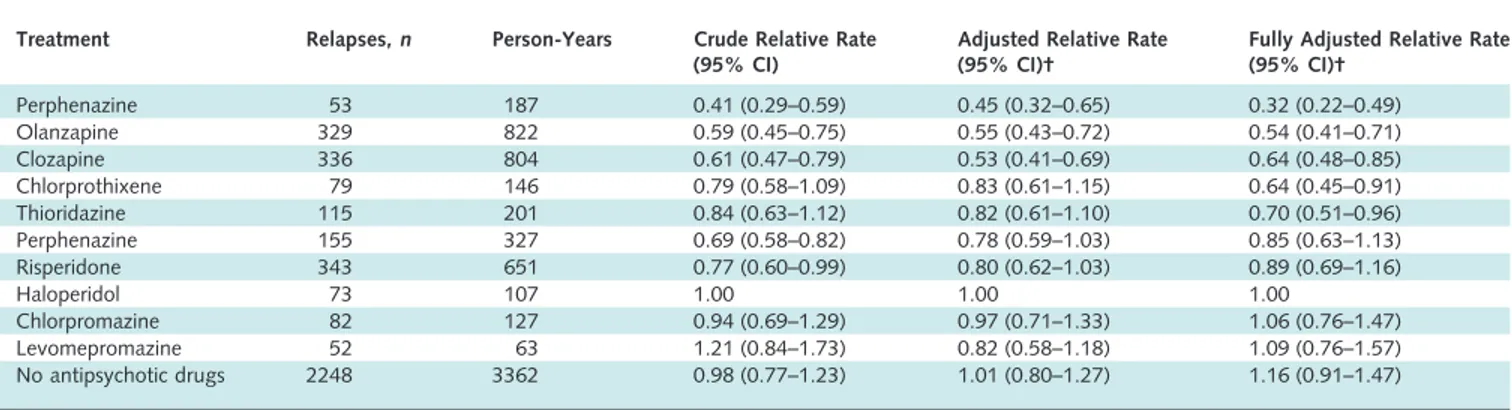
12 Statistical methods:
12(a) Describe all statistical methods, including those used to control for confounding.
Example
“The adjusted relative risk was calculated using the Mantel–Haenszel technique, when evaluating if confound-ing by age or gender was present in the groups compared. The 95% confidence interval (CI) was computed around the adjusted relative risk, using the variance according to Greenland and Robins and Robins et al.” (93).
Explanation
In general, there is no one correct statistical analysis but, rather, several possibilities that may address the same question but make different assumptions. Regardless, in-vestigators should predetermine analyses at least for the primary study objectives in a study protocol. Often addi-tional analyses are needed, either instead of, or as well as, those originally envisaged, and these may sometimes be motivated by the data. When a study is reported, authors should tell readers whether particular analyses were sug-gested by data inspection. Even though the distinction be-tween prespecified and exploratory analyses may sometimes be blurred, authors should clarify reasons for particular analyses.
cedures, data transformation, and calculations of attribut-able risks, should also be described. Nonstandard or novel approaches should be referenced, and the statistical soft-ware used reported. As a guiding principle, we advise sta-tistical methods be described “with enough detail to enable a knowledgeable reader with access to the original data to verify the reported results” (100).
In an empirical study, only 93 of 169 articles (55%) reporting adjustment for confounding clearly stated how continuous and multicategory variables were entered into the statistical model (101). Another study found that among 67 articles in which statistical analyses were ad-justed for confounders, it was mostly unclear how con-founders were chosen (4).
12(b) Describe any methods used to examine subgroups and interactions.
Example
“Sex differences in susceptibility to the 3 lifestyle-re-lated risk factors studied were explored by testing for bio-logic interaction according to Rothman: a new composite variable with 4 categories (a⫺b⫺, a⫺b⫹, a⫹b⫺, and a⫹b⫹) was redefined for sex and a dichotomous exposure of interest, wherea⫺ andb⫺ denote absence of exposure. RR was calculated for each category after adjustment for age. An interaction effect is defined as departure from ad-ditivity of absolute effects, and excess RR caused by inter-action (RERI) was calculated:
RERI⫽RR共a⫹b⫹兲⫺RR(a⫺b⫹)⫺RR(a⫹b⫺)⫺1
where RR(a⫹b⫹) denotes RR among those exposed to both factors where RR(a⫺b⫺) is used as reference category (RR⫽ 1.0). Ninety-five percent CIs were calculated as proposed by Hosmer and Lemeshow. RERI of 0 means no interaction” (103).
Explanation
As discussed in detail under item 17, many debate the use and value of analyses restricted to subgroups of the study population (4, 104). Subgroup analyses are neverthe-less often done (4). Readers need to know which subgroup analyses were planned in advance, and which arose while analyzing the data. Also, it is important to explain what methods were used to examine whether effects or associa-tions differed across groups (see item 17).
relative to no exposure, might be most informative. It is presented in the example for interaction under item 17, and the calculations on the different scales are explained in
Box 8.
12(c) Explain how missing data were addressed.
Example
“Our missing data analysis procedures used missing at random (MAR) assumptions. We used the MICE (multi-variate imputation by chained equations) method of mul-tiple multivariate imputation in STATA. We indepen-dently analysed 10 copies of the data, each with missing values suitably imputed, in the multivariate logistic regres-sion analyses. We averaged estimates of the variables to give a single mean estimate and adjusted standard errors accord-ing to Rubin’s rules” (106).
Explanation
Missing data are common in observational research. Questionnaires posted to study participants are not always filled in completely, participants may not attend all fol-low-up visits, and routine data sources and clinical data-bases are often incomplete. Despite its ubiquity and impor-tance, few papers report in detail on the problem of missing data (5, 107). Investigators may use any of several approaches to address missing data. We describe some strengths and limitations of various approaches in Box 6. We advise that authors report the number of missing val-ues for each variable of interest (exposures, outcomes, con-founders) and for each step in the analysis. Authors should give reasons for missing values if possible and indicate how many individuals were excluded because of missing data when describing the flow of participants through the study (see item 13). For analyses that account for missing data, authors should describe the nature of the analysis (for ex-ample, multiple imputation) and the assumptions that were made (for example, missing at random, seeBox 6).
12(d) Cohort study: If applicable, describe how loss to fol-low-up was addressed.
Example
“In treatment programmes with active follow-up, those lost to follow-up and those followed up at 1 year had similar baseline CD4 cell counts (median 115 cells perL and 123 cells perL), whereas patients lost to follow-up in programmes with no active follow-up procedures had con-siderably lower CD4 cell counts than those followed up (median 64 cells perL and 123 cells perL). . . . Treat-ment programmes with passive follow-up were excluded from subsequent analyses” (116).
Cohort studies are analyzed using life table methods or other approaches that are based on the person-time of fol-low-up and time to developing the disease of interest. Among individuals who remain free of the disease at the end of their observation period, the amount of follow-up time is assumed to be unrelated to the probability of de-veloping the outcome. This will be the case if follow-up ends on a fixed date or at a particular age. Loss to fol-low-up occurs when participants withdraw from a study before that date. This may hamper the validity of a study if loss to follow-up occurs selectively in exposed individuals, or in persons at high risk of developing the disease (“infor-mative censoring”). In the example above, patients lost to follow-up in treatment programs with no active follow-up had fewer CD4 helper cells than those remaining under observation and were therefore at higher risk of dying (116).
It is important to distinguish persons who reach the end of the study from those lost to follow-up. Unfortu-nately, statistical software usually does not distinguish be-tween the 2 situations: in both cases, follow-up time is automatically truncated (“censored”) at the end of the ob-servation period. Investigators therefore need to decide, ideally at the stage of planning the study, how they will deal with loss to follow-up. When few patients are lost, investigators may either exclude individuals with incom-plete follow-up, or treat them as if they withdrew alive at either the date of loss to follow-up or the end of the study. We advise authors to report how many patients were lost to follow-up and what censoring strategies they used.
12(d) Case– control study: If applicable, explain how match-ing of cases and controls was addressed.
Example
“We used McNemar’s test, paired t test, and condi-tional logistic regression analysis to compare dementia pa-tients with their matched controls for cardiovascular risk factors, the occurrence of spontaneous cerebral emboli, ca-rotid disease, and venous to arterial circulation shunt” (117).
Explanation
sim-plest form, the odds ratio becomes the ratio of pairs that are discordant for the exposure variable. If matching was done for variables like age and sex that are universal at-tributes, the analysis needs not retain the individual, per-son-to-person matching; a simple analysis in categories of age and sex is sufficient (50). For other matching variables, such as neighborhood, sibship, or friendship, however, each matched set should be considered its own stratum.
In individually matched studies, the most widely used method of analysis is conditional logistic regression, in which each case and their controls are considered together. The conditional method is necessary when the number of controls varies among cases, and when, in addition to the matching variables, other variables need to be adjusted for. To allow readers to judge whether the matched design was appropriately taken into account in the analysis, we recom-mend that authors describe in detail what statistical meth-ods were used to analyze the data. If taking the matching into account does have little effect on the estimates, au-thors may choose to present an unmatched analysis.
12(d) Cross-sectional study: If applicable, describe analytical methods taking account of sampling strategy.
Example
“The standard errors (SE) were calculated using the Taylor expansion method to estimate the sampling errors of estimators based on the complex sample design. . . . The overall design effect for diastolic blood pressure was found to be 1.9 for men and 1.8 for women, and for systolic blood pressure, it was 1.9 for men and 2.0 for women” (118).
Explanation
Most cross-sectional studies use a prespecified sam-pling strategy to select participants from a source popula-tion. Sampling may be more complex than taking a simple random sample, however. It may include several stages and clustering of participants (for example, in districts or vil-lages). Proportionate stratification may ensure that sub-groups with a specific characteristic are correctly repre-sented. Disproportionate stratification may be useful to oversample a subgroup of particular interest.
An estimate of association derived from a complex sample may be more or less precise than that derived from a simple random sample. Measures of precision, such as standard error or confidence interval, should be corrected using the design effect, a ratio measure that describes how much precision is gained or lost if a more complex sam-pling strategy is used instead of simple random samsam-pling (119). Most complex sampling techniques lead to a de-crease of precision, resulting in a design effect greater than 1.
may understand how the chosen sampling method influ-enced the precision of the obtained estimates. For instance, with clustered sampling, the implicit trade-off between eas-ier data collection and loss of precision is transparent if the design effect is reported. In the example, the calculated design effect of 1.9 for men indicates that the actual sample size would need to be 1.9 times greater than with simple random sampling for the resulting estimates to have equal precision.
12(e) Describe any sensitivity analyses.
Example
“Because we had a relatively higher proportion of ‘missing’ dead patients with insufficient data (38/148⫽ 25.7%) as compared to live patients (15/437⫽ 3.4%) . . . , it is possible that this might have biased the results. We have, therefore, carried out a sensitivity analysis. We have assumed that the proportion of women using oral contraceptives in the study group applies to the whole (19.1% for dead, and 11.4% for live patients), and then applied two extreme scenarios: either all the exposed miss-ing patients used second-generation pills or they all used third-generation pills” (120).
Explanation
Sensitivity analyses are useful to investigate whether the main results are consistent with those obtained with alternative analysis strategies or assumptions (121). Issues that may be examined include the criteria for inclusion in analyses, the definitions of exposures or outcomes (122), which confounding variables merit adjustment, the han-dling of missing data (120, 123), possible selection bias or bias from inaccurate or inconsistent measurement of expo-sure, disease, and other variables; and specific analysis choices, such as the treatment of quantitative variables (see item 11). Sophisticated methods are increasingly used to simultaneously model the influence of several biases or as-sumptions (124 –126).
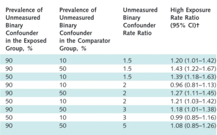
In 1959, Cornfield and colleagues famously showed that a relative risk of 9 for cigarette smoking and lung cancer was extremely unlikely to be due to any conceivable confounder, because the confounder would need to be at least 9 times as prevalent in smokers as in nonsmokers (127). This analysis did not rule out the possibility that such a factor was present, but it did identify the prevalence such a factor would need to have. The same approach was recently used to identify plausible confounding factors that could explain the association between childhood leukemia and living near electric power lines (128). More generally, sensitivity analyses can be used to identify the degree of confounding, selection bias, or information bias required to distort an association. One important, perhaps under-recognized, use of sensitivity analysis is when a study shows little or no association between an exposure and an
out-come and it is plausible that confounding or other biases toward the null are present.
Results
The Results section should give a factual account of what was found, from the recruitment of study partici-pants, the description of the study population, to the main results and ancillary analyses. It should be free of interpre-tations and discursive text reflecting the authors’ views and opinions.
13 Participants:
13(a) Report the numbers of individuals at each stage of the study— e.g., numbers potentially eligible, examined for eligi-bility, confirmed eligible, included in the study, completing follow-up, and analyzed.
Example
“Of the 105 freestanding bars and taverns sampled, 13 establishments were no longer in business and 9 were lo-cated in restaurants, leaving 83 eligible businesses. In 22 cases, the owner could not be reached by telephone despite 6 or more attempts. The owners of 36 bars declined study participation. . . . The 25 participating bars and taverns employed 124 bartenders, with 67 bartenders working at least 1 weekly daytime shift. Fifty-four of the daytime bar-tenders (81%) completed baseline interviews and spirome-try; 53 of these subjects (98%) completed follow-up” (129).
Explanation
Detailed information on the process of recruiting study participants is important for several reasons. Those included in a study often differ in relevant ways from the target population to which results are applied. This may result in estimates of prevalence or incidence that do not reflect the experience of the target population. For exam-ple, people who agreed to participate in a postal survey of sexual behavior attended church less often, had less conser-vative sexual attitudes and earlier age at first sexual inter-course, and were more likely to smoke cigarettes and drink alcohol than people who refused (130). These differences suggest that postal surveys may overestimate sexual liberal-ism and activity in the population. Such response bias (see
universally agreed definitions for participation, response, or follow-up rates, readers need to understand how authors calculated such proportions (134).
Ideally, investigators should give an account of the numbers of individuals considered at each stage of recruit-ing study participants, from the choice of a target popula-tion to the inclusion of participants’ data in the analysis. Depending on the type of study, this may include the number of individuals considered to be potentially eligible, the number assessed for eligibility, the number found to be eligible, the number included in the study, the number examined, the number followed up, and the number in-cluded in the analysis. Information on different sampling units may be required, if sampling of study participants is carried out in 2 or more stages as in the example above (multistage sampling). In case– control studies, we advise that authors describe the flow of participants separately for case and control groups (135). Controls can sometimes be selected from several sources, including, for example, hos-pitalized patients and community dwellers. In this case, we recommend a separate account of the numbers of partici-pants for each type of control group. Olson and colleagues proposed useful reporting guidelines for controls recruited through random-digit dialing and other methods (136).
A recent survey of epidemiologic studies published in 10 general epidemiology, public health, and medical jour-nals found that some information regarding participation was provided in 47 of 107 case– control studies (59%), 49 of 154 cohort studies (32%), and 51 of 86 cross-sectional studies (59%) (137). Incomplete or absent reporting of participation and nonparticipation in epidemiologic stud-ies was also documented in 2 other surveys of the literature (4, 5). Finally, there is evidence that participation in epi-demiologic studies may have declined in recent decades (137, 138), which underscores the need for transparent reporting (139).
13(b) Give reasons for nonparticipation at each stage.
Example
“The main reasons for nonparticipation were the par-ticipant was too ill or had died before interview (cases 30%, controls⬍ 1%), nonresponse (cases 2%, controls 21%), refusal (cases 10%, controls 29%), and other rea-sons (refusal by consultant or general practitioner, non-English speaking, mental impairment) (cases 7%, controls 5%)” (140).
Explanation
Explaining the reasons why people no longer partici-pated in a study or why they were excluded from statistical analyses helps readers judge whether the study population was representative of the target population and whether bias was possibly introduced. For example, in a cross-sec-tional health survey, nonparticipation due to reasons
un-likely to be related to health status (for example, the letter of invitation was not delivered because of an incorrect ad-dress) will affect the precision of estimates but will proba-bly not introduce bias. Conversely, if many individuals opt out of the survey because of illness or perceived good health, results may underestimate or overestimate the prev-alence of ill health in the population.
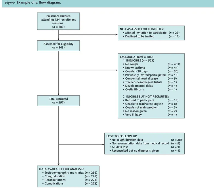
13(c) Consider use of a flow diagram.
Example
See theFigure.
Explanation
An informative and well-structured flow diagram can readily and transparently convey information that might otherwise require a lengthy description (142), as in the example above. The diagram may usefully include the main results, such as the number of events for the primary outcome. While we recommend the use of a flow diagram, particularly for complex observational studies, we do not propose a specific format for the diagram.
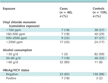
14 Descriptive data:
14(a) Give characteristics of study participants (e.g., demo-graphic, clinical, social) and information on exposures and potential confounders.
Example
SeeTable 1.
Explanation
Readers need descriptions of study participants and their exposures to judge the generalizability of the findings. Information about potential confounders, including whether and how they were measured, influences judg-ments about study validity. We advise authors to summa-rize continuous variables for each study group by giving the mean and standard deviation, or, when the data have an asymmetrical distribution (as is often the case), the median and percentile range (for example, 25th and 75th percen-tiles). Variables that make up a small number of ordered categories (such as stages of disease I to IV) should not be presented as continuous variables; it is preferable to give numbers and proportions for each category (seeBox 4). In studies that compare groups, the descriptive characteristics and numbers should be given by group, as in the example above.
con-Figure.Example of a flow diagram.
From reference 141.
Table 1. Characteristics of the Study Base at Enrollment, Castellana G (Italy), 1985–1986*
Characteristic HCV Negative
(nⴝ1458)
HCV Positive (nⴝ511)
Unknown (nⴝ513)
Sex,n (%)
Male 936 (64) 296 (58) 197 (39)
Female 522 (36) 215 (42) 306 (61)
Mean age at enrollment (SD),y 45.7 (10.5) 52.0 (9.7) 52.5 (9.8)
Daily alcohol intake,n (%)
None 250 (17) 129 (25) 119 (24)
Moderate† 853 (59) 272 (53) 293 (58)
Excessive‡ 355 (24) 110 (22) 91 (18)
*Adapted from reference 143. HCV⫽hepatitis C virus.
†Men,⬍60 g ethanol/d; women,⬍30 g ethanol/d.
founder that has a strong effect on the outcome can be important (144, 145).
In cohort studies, it may be useful to document how an exposure relates to other characteristics and potential confounders. Authors could present this information in a table with columns for participants in 2 or more exposure categories, which permits to judge the differences in con-founders between these categories.
In case– control studies, potential confounders cannot be judged by comparing cases and controls. Control per-sons represent the source population and will usually be different from the cases in many respects. For example, in a study of oral contraceptives and myocardial infarction, a sample of young women with infarction more often had risk factors for that disease, such as high serum cholesterol, smoking, and a positive family history, than the control group (146). This does not influence the assessment of the effect of oral contraceptives, as long as the prescription of oral contraceptives was not guided by the presence of these risk factors—for example, because the risk factors were only established after the event (seeBox 5). In case– con-trol studies, the equivalent of comparing exposed and non-exposed controls for the presence of potential confounders
(as is done in cohorts) can be achieved by exploring the source population of the cases: if the control group is large enough and represents the source population, exposed and unexposed controls can be compared for potential con-founders (121, 147).
14(b) Indicate the number of participants with missing data for each variable of interest.
Example
SeeTable 2.
Explanation
As missing data may bias or affect generalizability of results, authors should tell readers the amounts of missing data for exposures, potential confounders, and other im-portant characteristics of patients (see item 12c andBox 6). In a cohort study, authors should report the extent of loss to follow-up (with reasons), because incomplete follow-up may bias findings (see items 12d and 13) (148). We advise authors to use their tables and figures to enumerate amounts of missing data.
14(c) Cohort study: Summarize follow-up time— e.g., average and total amount.
Example
“During the 4366 person-years of follow-up (median 5.4, maximum 8.3 years), 265 subjects were diagnosed as having dementia, including 202 with Alzheimer’s disease” (149).
Explanation
Readers need to know the duration and extent of fol-low-up for the available outcome data. Authors can present a summary of the average follow-up with either the mean or median follow-up time or both. The mean allows a reader to calculate the total number of person-years by multiplying it with the number of study participants. Au-thors also may present minimum and maximum times or percentiles of the distribution to show readers the spread of follow-up times. They may report total person-years of fol-low-up or some indication of the proportion of potential data that was captured (148). All such information may be presented separately for participants in 2 or more exposure categories. Almost one half of 132 articles in cancer jour-nals (mostly cohort studies) did not give any summary of length of follow-up (37).
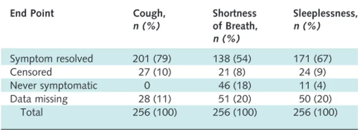
15 Outcome data
Cohort study: Report numbers of outcome events or summary measures over time.
Example
SeeTable 3. Table 2. Symptom End Points Used in Survival Analysis*
End Point Cough, n (%)
Shortness of Breath, n (%)
Sleeplessness, n (%)
Symptom resolved 201 (79) 138 (54) 171 (67)
Censored 27 (10) 21 (8) 24 (9)
Never symptomatic 0 46 (18) 11 (4)
Data missing 28 (11) 51 (20) 50 (20) Total 256 (100) 256 (100) 256 (100)
*Adapted from reference 141.
Table 3. Rates of HIV-1 Seroconversion by Selected Sociodemographic Variables, 1990 –1993*
Variable Person-Years Seroconverted, n
Rate/1000 Person-Years (95% CI)
Calendar year
1990 2197.5 18 8.2 (4.4–12.0)
1991 3210.7 22 6.9 (4.0–9.7)
1992 3162.6 18 5.7 (3.1–8.3)
1993 2912.9 26 8.9 (5.5–12.4)
1994 1104.5 5 4.5 (0.6–8.5)
Tribe
Bagandan 8433.1 48 5.7 (4.1–7.3)
Other Ugandan 578.4 9 15.6 (5.4–25.7)
Rwandese 2318.6 16 6.9 (3.5–10.3)
Other tribe 866.0 12 13.9 (6.0–21.7)
Religion
Muslim 3313.5 9 2.7 (0.9–4.5)
Other 8882.7 76 8.6 (6.6–10.5)