APPLICATION OF NEURAL NETWORKS TO CONDITION MONITORING AND
PREDICTION OF ACOUSTIC FATIGUE FAILURES
PACS REFERENCE:
Baranov Sergey Russian Aviation Co Ltd,
6 Leningradskoye Shosse, 125299 Moscow, Russia Tel/Fax: +7 (095) 158-2036
E-mail: [email protected]
ABSTRACT
Under consideration is condition monitoring of thin-walled structures, which suffer fatigue failures resulted from high-level wide-band loads in acoustic frequency range. Destructiveness is estimated with the aid of spectral characteristics of structure parameters measured in checkpoints. It was shown that Kohonen networks made it possible to diagnose a structure when neither all possible types of destruction nor the corresponding changes induced in the spectral characteristics were unpredictable in advance. The ways of reduction of input data dimension to improve the learning and operation network quality are described. The system of statistical goodness-of-fit tests for estimating the effectiveness of network functioning is proposed. Prediction of damage probabilities is carried out on the base of accumulated observations. Probability dynamics is described by continuous time, discrete state Markov processes. The method of minimum chi-square is used to identify unknown model characteristics by means of comparison of observed and expected histograms presenting damage distributions at the given time points.
INRODUCTION
Engine jet noise, pressure fluctuations in turbulent boundary layer and other high-level acoustic loads result in fatigue failures of aircraft structures and unacceptable level of on-board equipment damages. These problems have been attracting attention of researches since 50-s after numerous acoustic fatigue failures of aircraft resulted from increase of airspeed and change of engine types. Last years, the interest to this problem became stronger owing to development of new generation of supersonic airplanes and hypersonic flight vehicles.
Acoustic loads are the most dangerous for thin-walled aircraft structures. They are wide-band (up to 5000 Hz) random process, with level varying from 145 to 170 dB in different points of aircraft surface.
opportunity to cut down expenses for aircraft maintenance, raise the reliability of destruction monitoring and simplify the routine maintenance.
MODELS AND METHODS
According to the described approach, destructiveness is estimated by the changes of distributed structure stiffness, which is, in its turn, recognized by the qualitative changes of normalized parameter spectral characteristics measured in checkpoints. Normalizing makes it possible to analyze only qualitative structure response and not to take into account the level of load.
Such an approach based on the estimation of averaged structure properties seems more promising than the search of separate cracks [1,2], which are not always accessible for direct observation and hard to predict because of considerable dispersion in their evolution. The use of secondary characteristics (such as spectra) instead of time-domain realizations as check data is caused by the following facts:
• spectra keep sufficient amount of useful information about the process under study; • spectra need less memory in digital form of representation;
• spectra may be easily and quickly computed with controlled accuracy.
Components of the technology used for monitoring of fatigue failures are presented in Figure 1.
STRUCTURE MOTION
SPECTRA (in checkpoints)
REDUCING PROBLEM DIMENSION (principal components or factor analysis)
NEURAL NETWORK MODELING (supervised learning)
NEURAL NETWORK MODELING (unsupervised learning)
0 0 . 1 0 . 2 0 . 3 0 . 4 0 . 5 0 . 6 0 . 7 0 . 8 0 . 9 1
0 5 0 0 1000 1500 2000 2500 3000
[image:2.612.102.557.317.666.2]O K Only 1 Only 2 Panel Nonlin
Figure 1. Components of the technology used for monitoring and prediction of fatigue failures.
χ
2χ
2PREDICTION OF DAMAGE PROBABILITIES
(on the base of Markov models)
STATISTICAL ANALYSIS OF RESULTS
Since all the damages are not assumed to be known before diagnostics, it is impossible to apply ordinary neural networks with supervised learning for their detection. Self-organizing feature maps, or Kohonen networks [3, 4], for which output variables are not required, may be useful in this case. A self-organizing feature map may be used as a detector of new events: it informs about input case rejection only if this case differs from all labeled radial units significantly (more than a given acceptance distance for radial units). Simultaneous application of different networks duplicating each other makes it possible to improve the recognition quality [5].
When all variants of system damages are known before, the problem is essentially simpler. One can employ traditional neural networks with supervised learning (perceptrons, radial basis function networks, etc.). The output of a classifying network is represented with the aid of a nominal variable according to the scheme “One-of-N”. In both approaches, frequency ranges are used as input variables and ordered lists of values of normalized power spectra densities at their centers – as observations. So, each input observation represents a separate spectrum.
If the number of accountable frequency ranges is such a great one that it not only degrades network performances but excessively enlarges the size of training data [6], problem dimension may be reduced. Some hypothetical latent variables, which explain initial data fluctuations with acceptable errors, are thereto determined and used later as input data. Either factor or principal component analysis [7] may be applied here. In case of factor analysis, latent variables (factors) are selected to obtain the best (from the viewpoint of a given criterion) approximation of correlation or covariance matrices calculated for observed variables. In case of principal component analysis, a subspace of smaller dimension laying on the eigenvectors of initial correlation (covariance) matrix and explaining sufficiently great part of total observed variance (as a rule, more than 80%) is determined.
To get stable output of factor or component analysis applied to power spectral densities considered here, mean values for each observed variable should be kept fixed (for example, they may be equal to zero) at any number of cases. It is convenient to use the following formal technique: to double the given set of cases before calculation of latent variables supplementing it with initial power spectral densities signed with “minus” (so as each value of an observed variable has the double yielding zero sum with itself) and, then, to carry out the mentioned analysis for these extended data.
Reducing problem dimension makes it possible to decrease the number of units in recognizing networks and yields significant advantages: smaller networks need smaller samples for their training, have better ability for generalization, etc. Reducing dimension is an alternative to immediate selection of input data on the base of sensitivity analysis. It not only eliminates the information redundancy but also reveals internal dependencies between variables.
Estimations of classification quality, which are based on the percentage of correct cases in the verification set only, may not be considered as acceptable ones since they do not take into account amount of sampling and differences in the output resulted from training and verification sets. More reliable estimations based on statistical goodness-of-fit tests may be carried out when the following criteria are verified [8]:
1) hypothesis of absence of statistically significant differences between predicted and observed output obtained for the verification set,
2) hypothesis of absence of statistically significant differences between classification carried out on the training and verification sets,
3) equivalence hypotheses for distributions of different input data types in training and verification sets.
Prediction is carried out on the base of accumulated observations. Probability dynamics is described by continuous time, discrete state Markov processes. The given damage types are considered as separate discrete states in which the analyzed system has some probability to find itself. In due course transitions between the states are the case.
It is assumed that state-to-state transitions (corresponding to each branch of the graph) meet the properties of Poisson’s flows of events.
The method of chi-square minimum is used to identify independent model parameters (transition flow rates) on the base of observation results. For the problems under consideration, it usually yields estimations, which are close to ones of the maximum likelihood method. According to the presented approach, this statistic is minimized at the specified time points in which observed data are available.
Obtained values of free parameters are considered as fatigue failure characteristics, which have become apparent during observations.
The same criteria may be also used to compare different Markov models for selecting their optimal variant.
EXAMPLE OF PREDICTION
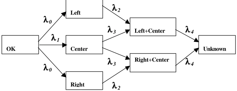
Prediction results are demonstrated by the example of fatigue failures of an air-intake panel. Recognized are the following structure conditions: OK - safe structure; Center – 1 weld in the panel center has been damaged; Left - 2 welds in the left part of the panel have been damaged; Right - 2 welds in the right part of the panel have been damaged.
The diagram presented in Figure 2 may be used to estimate damage probabilities. It represents mutual coupling between different damage types. All the damages that have not been described before correspond to the state Unknown. Distribution of flow rates takes into account the system symmetry.
Probabilities of being in different states as functions of time are defined by the following set of Kolmogorov ordinary differential equations (
p
i is probability of being in state Noi
):.
p
ë
p
ë
dt
dp
,
p
ë
p
ë
p
ë
dt
dp
,
p
ë
p
ë
p
ë
dt
dp
,
p
ë
p
ë
dt
dp
,
p
2ë
p
ë
dt
dp
,
p
ë
p
ë
dt
dp
,
p
ë
p
2ë
dt
dp
5
4
4
4
6
5
4
2
3
3
2
5
4
4
2
3
1
2
4
3
2
0
0
3
2
3
0
1
2
1
2
0
0
1
0
1
0
0
0
+
=
−
+
=
−
+
=
−
=
−
=
−
=
−
−
=
To integrate these equations, one has to assign initial conditions:
.
)
(
...
)
(
)
(
,
)
(
0
1
10
20
60
0
0
=
p
=
p
=
p
=
[image:4.612.129.520.350.501.2]p
Final values of state probabilities
p
0,
p
1,...,
p
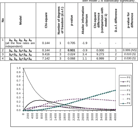
6 determined by numerical integration at the specified time points may be considered as functions of free parameters. These values agree with an exact solution to the precision of the numerical integration, which may be set arbitrarily small. [image:5.612.90.532.243.653.2]Statistical criteria make it possible to optimize the model selecting that sort of ratios between flow rates, which yield the best matching with the observation results. Corresponding estimations for different variants of the model presented in Figure 2 are shown in Table 1. The chi-square criterion is used here to compare different variants of models, viz.: goodness-of-fit measure for the full model (model 1) is confronted with the analogous characteristic of reduced models. Since difference in the values of chi-square criteria for the full and reduced models is itself distributed as chi-square, it is used to figure out whether simplifications are statistically significant or not [5, 8]. Table 1 shows that models 1 and 2 are the best fitted with regard to observations. Model 2 is preferable as it is simpler.
Table 1. Model fitting for damage distribution after 2000 exploitation hours (the model is presented in Figure 2; NS –difference with model 1 is not statistically significant, S –difference with model 1 is statistically significant) .
No
Model
Chi
-square
Number of degrees of freedom (d.o.f.)
p
-value
Akaike information
criterion
Chi
-square
diffe
rence
(comparison with
model 1)
D.o.f. difference
p
-value for difference
1 λλ0, λλ1, λλ2, λλ3, λλ4
(all the flow rates are independent)
0.144 1 0.705 -1.9 - - -
2 λλ0, λλ1, λλ2=λλ3, λλ4 0.144 2 0.931 -3.9 0.000 1 0.999 (NS) 3 λλ0=λλ1, λλ2=λλ3, λλ4 9.416 3 0.024 3.4 9.273 2 0.010 (S) 4 λλ0, λλ1, λλ2=λλ3=λλ4 7.142 3 0.068 1.1 6.999 2 0.030 (S)
Predicted probabilities of being in different system states (as functions of time) are given in Figure 3.
Figure 3. Predicted probabilities of being in states P0, P1, …, P6 as functions of time.
0.0 0.1 0.2 0.3 0.4 0.5 0.6 0.7 0.8 0.9 1.0
0
200 400 600 800
1000 1200 1400 1600 1800 2000 2200 2400 2600 2800 3000 3200 3400 3600 3800 4000 Â ð å ì ÿ , ÷ à ñ û
Âåðîÿòíîñòü
It was shown in paper [8] that Markov models under the given inverse problem formulation are used as specialized neural networks. In this case states are analogues of neurons, activation functions are expressed via differential equations, transition flow rates are used as weights, and state probabilities are inputs and outputs of network units.
CONCLUSIONS
1. Analysis of spectral characteristics of parameters measured in checkpoints with the aid of neural networks makes it possible to estimate the character of fatigue failures of thin-walled aircraft structures suffered acoustic loading. The use of spectral characteristics saves on computer resources keeping sufficient amount of useful information about the process under study.
2. Kohonen networks (self-organizing feature maps) make it possible to diagnose fatigue failures in situations where neither all possible damage types nor corresponding changes induced in observed spectral characteristics are not predictable beforehand.
3. If all types of system damages are known beforehand, traditional neural networks with supervised learning (perceptrons, radial basis function networks) may be used for diagnostics. 4. Reduction of problem dimension (with the aid of principal component analysis, etc.) improves
characteristics of network training.
5. Presented statistical goodness-of-fit tests are necessary to estimate obtained network quality. 6. Parametric models described by continuous time, discrete state Markov processes make it
possible to predict probabilities of damage appearance as functions of time. Prediction is carried out by means of calculation of transition flow rates, which yield solutions best-fitting the observation data, and integration of Kolmogorov set of differential equations. These models under the given inverse problem formulation are used as specialized neural networks.
REFERENCES
1. C. Brousset and G. Baudrillard, Neural network for automating diagnosis in aircraft inspection,
Review of Progress in Quantitative Nondestructive Evaluation (Ed. By D. O. Thompson and D.
E. Chimenti), Plenum Press, New York, 12, 797-802, 1993.
2. R. M. V. Pidaparti and M. J. Palakal, Neural network approach to fatigue-crack-growth predictions under aircraft spectrum loadings, Journal of Aircraft 32, 825-831, 1995.
3. T. Kohonen, Improved versions of learning vector quantization, Proc. International Joint
Conference on Neural Networks 1, San Diego, USA, 1990.
4. T. Kohonen, Self-organized formation of topologically correct feature maps, Biological
Cybernetics 43, 59-69, 1982.
5. S. N. Baranov and L. S. Kuravsky, Acoustic vibrations: modeling, optimization and diagnostics, Moscow: RUSAVIA, 2001 (in Russian).
6. A. I. Galushkin, Neural network theory, Moscow: IPRZhR, 2000 (in Russian).
7. D. N. Lawley and A. E. Maxwell, Factor Analysis as a Statistical Method, Moscow: Mir, 1967. 8. Kuravsky L. S., Baranov S. N., Application of neural networks for diagnostics and forecasting of