Comportamiento resistente al deslizamiento de geosintéticos (Shear strength behaviour of geosynthetics)

(1)

UNIVERSIDAD DE CANTABRIA

ESCUELA TÉCNICA SUPERIOR DE INGENIEROS

DE CAMINOS, CANALES Y PUERTOS

DEPARTAMENTO DE CIENCIA E INGENIERÍA DEL TERRENO Y DE LOS MATERIALES

TESIS DOCTORAL

COMPORTAMIENTO RESISTENTE AL DESLIZAMIENTO

DE GEOSINTÉTICOS

Autora

ANA BELÉN MARTÍNEZ BACAS

Directores

JORGE CAÑIZAL BERINI HEINZ KONIETZKY

(2)

(3)

Esta tesis doctoral ha sido financiada por las siguientes empresas e instituciones:

- Proyecto de investigación “Estudio de las características friccionales de los geosintéticos empleados en vertederos”, Financiado por la empresa CESPA del GRUPO FERROVIAL.

- Este proyecto obtuvo una subvención PROFIT 2006. FIT-310200-2006-57 del MINISTERIO DE INDUSTRIA, TURISMO Y COMERCIO, en el Programa Nacional de Ciencias y Tecnología Medioambientales dentro del Subprograma Nacional de Tecnologías para la Gestión Sostenible Medioambiental

- Universidad de Freiberg (Bergakademie Freiberg, Alemania), Departamento de Mecánica de Rocas (Gebirgs-und Felsmechanik/Felsbau).

- Beca de Investigación Doctoral del Gobierno alemán, Deutscher Akademischer Austausch Dienst (DAAD) (convocatoria año 2008)

(4)

(5)

Agradecimientos/Dank

Deseo expresar mi sincero agradecimiento al Prof. Jorge Cañizal, director de esta tesis, por todo su conocimiento y experiencia compartida, así como su esfuerzo y tiempo aportados. Agradecerle también la oportunidad que me ha dado de abrir la ventana a la investigación, que espero que siga siendo parte de mi actividad profesional en el futuro.

Meinen allerherzlichsten Dank gilt Herrn Professor Konietzky, dem Direktor der Thesis, der es mir ermöglichte einen Teil der Forschungsarbeit am Institut für Felsmechanik an der Technischen Universität Bergakademie Freiberg auszuführen. Sein umfangreiches Wissen und seine Erfahrung waren der Schlüssel für die Entwicklung dieser Arbeit. Vielen Dank Professor für die Zeit, die Sie mir gewidmet haben, für die Besprechungen und Diskusionen, die wir unterhielten und deren Ergebnis das vierte Kapitel, der vorliegenden Thesis ist, auf die ich sehr stolz bin.

Del mismo modo, deseo transmitir mi agradecimiento al Prof. César Sagaseta, por la ayuda que me ha prestado, por lo que me ha enseñado, así como por sus consejos y recomendaciones.

También agradecer a la Prof. ª Almudena Da Costa toda la ayuda y enseñanza prestada, además de su apoyo y compresión.

Igualmente quiero expresar mi gratitud a la empresa CESPA del Grupo Ferrovial, que me han sufragado económicamente, otorgándome una beca de investigación a través de la Universidad de Cantabria. Agradeciendo especialmente a Mónica Fernández, del Departamento I+D+i, y Ángel Martínez, del Departamento de Depósitos Controlados, por todo el apoyo logístico, conocimientos técnicos y ayuda recibido.

Agradecimiento especial al personal del Laboratorio de Geotecnia de la Universidad de Cantabria, Javier de la Fuente y Fernando del Puerto, porque sin su ayuda y dedicación difícilmente se podría haber llevado a cabo el trabajo experimental de esta investigación.

(6)

(7)

Índice de contenidos

Lista de Figuras 13

Lista de Tablas 21

Notación 23

Resumen 25

Abstract 27

Thesis summary 29

Presentación del documento 47

Introducción 49

1 Estado del conocimiento 57

1.1 Sección básica de un vertedero 57

1.2 Tipos de geosintéticos 59

1.3 Sistemas de protección de vertederos: vaso y sellado 61

1.4 Estudio de la estabilidad de vertederos de residuos sólidos urbanos 64

1.5 Obtención de los parámetros resistentes al corte de los residuos 71

1.6 Obtención de los parámetros resistentes al corte de las interfaces entre

geosintéticos y entre suelo y geosintético 73

1.7 Modelos de comportamiento de las discontinuidades 83

1.8 Consideraciones finales 95

2 Metodología del ensayo de corte directo para las interfaces

geosintético/geosintético y suelo/geosintético 97

2.1 Introducción 97

2.2 Limitaciones y problemas encontrados en la aplicación de los métodos

de sujeción de geosintéticos preexistentes 98

2.3 Descripción y uso del nuevo sistema de sujeción de geosintéticos 101

2.3.1 Características 101

2.3.2 Desarrollo 101

(8)

2.4 Sistemas de sujeción adoptados para los diversos geosintéticos 104

2.5 Metodología desarrollada para la realización del ensayo 105

2.5.1 Guía de ensayo 105

2.5.2 Compactación del suelo 106

2.5.3 Esquema de ensayo para las diferentes interfaces 107

2.5.4 Condiciones de humedad del ensayo 109

2.6 Interpretación del ensayo 110

2.6.1 Ajuste mediante el modelo de Coulomb 112

2.6.2 Otros posibles modelos de ajuste 113

3 Análisis de resultados de los ensayos de corte directo de las interfaces 115

3.1 Consideraciones generales 115

3.2 Materiales utilizados en el programa de ensayos de laboratorio 117

3.3 Interfaz geomembrana/geotextil 121

3.3.1 Comportamiento resistente al corte de la interfaz 122 3.3.2 Influencia de las condiciones de humedad del ensayo en la

resistencia al corte de la interfaz 126

3.3.3 Influencia de la rugosidad de la geomembrana en la resistencia

al corte de la interfaz 127

3.3.4 Influencia del tipo de geotextil en la resistencia al corte de la

interfaz 134

3.3.5 Comparación de los resultados obtenidos con otros autores 141

3.4 Interfaz geomembrana/geocompuesto drenante 147

3.4.1 Comportamiento resistente al corte de la interfaz 147 3.4.2 Influencia de la rugosidad de la geomembrana en la resistencia

3.4.3 Influencia de la masa por unidad de área del geotextil en contacto con la geomembrana en la resistencia al corte de la

interfaz 156

3.4.4 Influencia de la geored en la resistencia al corte de la interfaz 157

3.5 Interfaz geomembrana/suelo 158

3.5.1 Comportamiento resistente al corte de la interfaz 159 3.5.2 Influencia de la rugosidad de la geomembrana en la resistencia

(9)

3.6 Interfaz geotextil/suelo 164 3.6.1 Comportamiento resistente al corte de la interfaz 165 3.6.2 Influencia del tipo de suelo en la resistencia al corte de la

interfaz 166

3.6.3 Influencia de las condiciones de humedad del ensayo en la

3.6.4 Influencia del tipo de geotextil en la resistencia al corte de la

interfaz 169

3.7 Interfaz geomembrana/Geosynthetic Clay Liner 170

3.7.1 Comportamiento resistente al corte de la interfaz 170 3.7.2 Influencia de las condiciones de humedad del ensayo en la

3.7.3 Influencia de la rugosidad de la geomembrana en la resistencia

3.8 Interfaz geocompuesto drenante/Geosynthetic Clay Liner 177

3.8.1 Comportamiento resistente de la interfaz 178

3.8.2 Influencia de las condiciones de humedad del ensayo en la

3.8.3 Influencia del tipo de geocompuesto drenantes en la resistencia

3.9 Geosynthetic Clay Liner 183

3.9.1 Comportamiento resistente al corte de la GCL 183

3.10 Interfaz suelo/geomalla/geocompuesto drenante 186

3.10.1 Comportamiento resistente al corte de la interfaz 187 3.10.2 Influencia del tipo de geomalla en la resistencia al corte de la

interfaz 190

4 Model and numerical analysis of the direct shear test of

geomembrane/geotextile interface 193

4.1 Shear strength model 193

4.1.1 Theory 193

4.1.2 Modelling material 200

4.1.3 Residual friction angle (φ_r) 201

4.1.4 Geotextile reference compression stress (GCS) 203

4.1.5 Hook and Loop (HL) 207

(10)

4.1.7 Peak displacement (δ_peak) 214 4.1.8 Mobilization of hook and loop during shear 216 4.1.9 Normal stiffness (kn) and shear stiffness (ks). 219

4.1.10 Comparison with measured data 220

4.2 Numerical analysis 226

4.2.1 Steps to perform the Geomembrane/geotextile direct shear

model 226

4.2.2 Interpretation of results 236

4.2.3 How obtain the constants of the direct shear model? 238

4.2.4 Comparison with measured data 240

4.2.5 Different analysis of the direct shear numerical model

changing the geometry, initial and boundary conditions 242

Conclusiones y trabajo futuro 247

Conclusions and future research 257

Referencias 265

Apéndice A. Metodología y máquina de corte directo 273

Apéndice B. Resultados de ensayos de laboratorio 297

Apéndice C. Summary of parameters 451

Apéndice D. Spreadsheet of the shear strength model 459

Apéndice E. Summary of shear strength model results 461

(11)

13

Lista de figuras

Figura 1.1 Sección transversal de un vertedero de residuos sólidos urbanos (RSU) 58 Figura 1.2 Vista aérea del vertedero de Meruelo (Cantabria) 58

Figura 1.3 Tipos de geosintéticos 60

Figura 1.4 Secciones sistema impermeabilización y sellado de un vertedero de

RSU 63

Figura 1.5 Colocación de láminas de GCL en la base de un vertedero 63 Figura 1.6 Colocación de geomembranas y geotextiles en la base de un vertedero 64

Figura 1.7 Rotura a través de la masa de residuo 66

Figura 1.8 Deslizamiento a través de las láminas de impermeabilización 67

Figura 1.9 Inestabilidad a través del residuo 68

Figura 1.10 Inestabilidad en sistemas de impermeabilización y sellado 69 Figura 1.11 Inestabilidad dentro del sistema de impermeabilización 69 Figura 1.12 Parámetros recomendados para residuos. Sánchez et al. (1993) 73

Figura 1.13 Esquema del ensayo de corte directo 74

Figura 1.14 Pullout test, Fox et al. (1997) 75

Figura 1.15 Esquema aparato de corte "Pullout box". Mitchell et al. (1990) 75 Figura 1.16 Esquema del ensayo de plano inclinado. UNE-EN ISO 12957-2 76

Figura 1.17 Esquema del ensayo de corte anular 77

Figura 1.18 Envolventes y mecanismos de rotura muestras con superficies

irregulares. Modelo de Patton (1966) 84

Figura 1.19 Criterio de Barton (1973) para planos de discontinuidad en rocas 86 Figura 1.20 Primera clasificación y predicción de la resistencia al corte de tres

tipos de juntas rugosas (Barton, 1973) 87

Figura 1.21 Idealización de una superficie de discontinuidad (Plesha, 1987) 88 Figura 1.22 Gráfica log σn vs ΔVj para diferentes tipos de juntas (Bandis et al.,

1983) 90

Figura 1.23 Compresión de una junta, σi es la tensión inicial de la junta 90 Figura 1.24 Gráficas lineales de ΔV_j σ_n vs ΔV_j, junta de caliza, (Bandis et al.,

(12)

Figura 1.25 Variación de la rigidez a cortante de pico con la tensión normal de

diferentes tipos de juntas (Bandis et al., 1983) 93 Figura 1.26 Curva idealizada tensión tangencial-desplazamiento. Amadei et al.

(1998) 93

Figura 1.27 Comparación entre los resultados de experimentos de laboratorio y el

modelo constitutivo propuesto, Grasselli y Egger (2003) 94

Figura 2.1 Aparato de corte directo utilizado 98

Figura 2.2 Esquema del ensayo de corte directo (ASTM D5321-02) 99 Figura 2.3 Método de sujeción con papel de lija. Aspecto después del ensayo 100

Figura 2.4 Método de sujeción “truss plates” 100

Figura 2.5 Descripción de la placa dentada 102

Figura 2.6 Placa metálica dentada 103

Figura 2.7 Descripción del soporte metálico 103

Figura 2.8 Piezas del soporte metálico 104

Figura 2.9 Esquema ensayo corte directo tipo 1 108

Figura 2.13 Esquema del ensayo y resultados obtenidos 111

Figura 2.14 Envolventes de rotura bilineales, interfaz

geocompuesto/geomembrana 112

Figura 2.15 Envolventes de rotura curvas para una interfaz geotextil/geomembrana 114

Figura 3.1 Rugosidad de la geomembrana 117

Figura 3.2 Fotografías de varios métodos de fabricación de geotextiles 118 Figura 3.3 Esquema de la sección transversal de un geotextil agujeteado 119

Figura 3.4 Geocompuesto drenante 119

Figura 3.5 Esquema de la sección transversal de la GCL 120

Figura 3.6 Tipos de geomallas 120

Figura 3.7 Comportamiento resistente de la interfaz geomembrana

rugosa/geotextil 122

(13)

15

Figura 3.9 Esquema del mecanismo de interacción de la interfaz geomembrana rugosa/geotextil para a) valores bajos de la tensión normal y b)

valores altos de la tensión normal (después de Hebeler et al., 2005) 125 Figura 3.10 Daños observados en los geotextiles: a) GT3 b) GT1 126 Figura 3.11 Comparación de las envolventes de rotura de ensayos realizados en

condiciones húmedas y secas con la interfaz geomembrana/geotextil 127 Figura 3.12 Comparación envolventes de rotura con geomembrana lisa y rugosa 128 Figura 3.13 Las fotos 1 y 2 muestran respectivamente la planta y el alzado de la

macrotextura. En la foto 3 se observa el alzado de la microtextura 129 Figura 3.14 Efecto del tamaño de la macrotextura en la resistencia al corte de la

interfaz geomembrana rugosa/geotextil 129

Figura 3.15 Efecto de la macrotextura > 1 mm en la forma de la curva tensión

tangencial-desplazamiento horizontal 131

Figura 3.16 Comportamiento resistente de la interfaz GMr1/GT1 131 Figura 3.17 Efecto de la densidad de macrotextura en la resistencia al corte de las

interfaces geomembrana rugosa/geotextil 132

Figura 3.18 Imágenes tres tipos de geomembranas con tamaño rugosidad <1 mm 133 Figura 3.19 Envolventes rotura interfaz geomembrana rugosa/geotextil (GT1) 133 Figura 3.20 Variación del coeficiente de rozamiento con el tamaño de la rugosidad

para el geotextil GT1 134

Figura 3.21 Comparación de envolventes de rotura geomembrana lisa/geotextil 135 Figura 3.22 Efecto de la longitud de fibra del geotextil 136 Figura 3.23 Sensibilidad del geotextil agujeteado de fibra larga (GT1) 137 Figura 3.24 Sensibilidad del geotextil agujeteado de fibra corta (GT2) 138 Figura 3.25 Variación de la sensibilidad con el tamaño de la macrorugosidad

(geotextiles agujeteados) 138

Figura 3.26 Sensibilidad del geotextil termosoldado (GT3) 139 Figura 3.27 Variación de la sensibilidad con el tamaño de la macrorugosidad,

geotextil agujeteado (GT1) y termosoldado (GT3) 140 Figura 3.28 Efecto del método de fabricación del geotextil 140 Figura 3.29 Envolventes de rotura de las interfaces geomembrana/geotextil(GT3) 141 Figura 3.30 Comparación entre tensiones tangenciales de pico. Tamaño de

(14)

Figura 3.31 Comparación entre tensiones tangenciales post-pico. Tamaño de

muestras grande. a) σn < 500 kPa, b) σn < 100 kPa 144

Figura 3.32 Comparación de tensiones tangenciales pico. Tamaño de muestras

pequeño. a) σn < 500 kPa, b) σn < 100 kPa 145

Figura 3.33 Comparación de tensiones tangenciales post-pico. Tamaño de

muestras pequeño. a) σn < 500 kPa, b) σn < 100 kPa 146

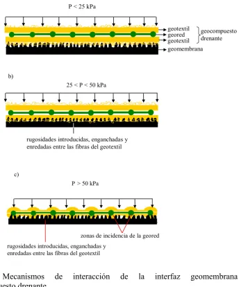
Figura 3.34 Comportamiento resistente de la interfaz geomembrana/geocompuesto 149 Figura 3.35 Mecanismos de interacción de la interfaz geomembrana

rugosa/geocompuesto drenante. 150

Figura 3.36 Comparación envolventes de rotura geomembrana lisa y rugosa 151 Figura 3.37 Envolventes de rotura de la interfaz

geomembrana/geocompuesto(GC1) 153

Figura 3.38 Sensibilidad de la interfaz geomembrana/geocompuesto(GC1) 153 Figura 3.39 Envolventes de rotura de la interfaz geomembrana/geocompuesto(GC2) 154 Figura 3.40 Sensibilidad de la interfaz geomembrana/geocompuesto(GC2) 154 Figura 3.41 Daños que se producen en las muestras ensayadas al corte 155 Figura 3.42 Envolventes de pico para diferente masa por unidad de área del

geotextil 156

Figura 3.43 Envolventes post-pico, diferente masa por unidad de área de geotextil 157 Figura 3.44 Envolventes de rotura. GMr2_s1/GC1 y GMr2_s1/geotextil 158 Figura 3.45 Comportamiento resistente de la interfaz geomembrana/suelo1 159 Figura 3.46 Daños producidos en la geomembrana lisa después del corte 160 Figura 3.47 Sensibilidad de la interfaz geomembrana/suelo1 160 Figura 3.48 Interacción suelo1-geomembrana (rugosidad mayor de 1 mm) 161 Figura 3.49 Interacción suelo1-geomembrana (rugosidad menor de 1 mm) 162 Figura 3.50 Envolventes de rotura de las interfaces geomembrana lisa/suelo1 y

geomembrana rugosa/suelo1 163

Figura 3.51 Envolventes de rotura de las interfaces geomembrana/suelo1 y de

resistencia interna del suelo1 164

(15)

17

Figura 3.56 Envolventes de la interfaz GT5/suelo1. Condiciones húmedas y secas 168 Figura 3.57 Muestras después del ensayo de corte directo. Foto a) en condiciones

secas. Foto b) en condiciones húmedas 168

Figura 3.58 Envolventes rotura para dos tipos de geotextil e interna del suelo. 169 Figura 3.59 Comportamiento al corte de la interfaz GMr3/GCL. Condiciones secas 171

Figura 3.60 Huellas en la superficie de la GCL 172

Figura 3.61 Mecanismo interacción geomembrana/GCL 172

Figura 3.62 Muestra de GCL ensayada: a) ensayo en condiciones secas b) ensayo

en condiciones húmedas 173

Figura 3.63Sensibilidad de la interfaz geomembrana/GCL 173 Figura 3.64 Comportamiento de la interfaz GMr3/GCL. Condiciones húmedas 174 Figura 3.65 Envolventes de rotura de la interfaz GMr3/GCL 175 Figura 3.66 Envolventes de rotura geomembrana/GCL y GCL sola: (a) en

condiciones secas y (b) húmedas 176

Figura 3.67 Efecto del tipo de rugosidad. Interfaz geomembrana/GCL 177 Figura 3.68 Comportamiento de la interfaz geocompuesto(GC3)/GCL en

condiciones secas 178

Figura 3.69 Sensibilidad de la interfaz geocompuesto/GCL 179 Figura 3.70 Condiciones húmedas. Interfaz geocompuesto(GC3)/GCL 180 Figura 3.71 Envolventes de rotura. Interfaz geocompuesto (GC3)/GCL 181 Figura 3.72 Plano de deslizamiento en condiciones secas 181 Figura 3.73 Plano de deslizamiento en condiciones húmedas 182 Figura 3.74 Efecto del tipo de geocompuesto drenante. Interfaz

geocompuesto/GCL 183

Figura 3.75 Comportamiento resistente de la GCL en condiciones secas 184 Figura 3.76 Muestra de GCL después de ser ensayada en condiciones secas 184 Figura 3.77 Comportamiento resistente de la GCL en condiciones húmedas 185 Figura 3.78 Muestra de GCL después de ser ensayada en condiciones húmedas 186 Figura 3.79 Envolventes de rotura de la GCL en condiciones secas y húmedas 186 Figura 3.80 Comportamiento de la interfaz suelo/geomalla/geocompuesto drenante 187 Figura 3.81 Muestras del ensayo suelo/geomalla/geocompuesto después de ser

ensayadas: a) geomalla1, b)geomalla2 188

Figura 3.82 Mecanismos de interacción suelo/geomalla/geocompuesto. Sección

(16)

Figura 3.83 Interacción suelo-geomalla. Sección paralela a la dirección de

desplazamiento de corte. 190

Figura 3.84 Envolventes de rotura interfaz suelo/geomalla/geocompuesto drenante 191 Figura 3.85 Dilatancia interfaz suelo/geomalla/geocompuesto 192

Figure 4.1 (a) Non-planar rock joint (Barton, 1973). (b) NWNP

geotextile/textured geomembrane interface (Hebeler et al., 2005) 193 Figure 4.2 (a) Examples of the range of joint roughnesses (Barton and Choubey,

1977). (b) Surfaces roughness of the geosynthetics 194 Figure 4.3 (a) Shear stress-displacement data obtained from replicas of rock joints

(Barton et al., 1985). (b) Shear stress-displacement data obtained from

texture geomembrane/geotextile interface. 194

Figure 4.4 Two methods for presenting the results of direct shear test on rock

joints. (Barton, 1973) 196

Figure 4.5 Sketch of interaction mechanisms between needle-punched non-woven geotextiles and textured geomembranes at different normal stresses:

(a) low normal stress and (b) high normal stress. (Hebeler et al., 2005) 197 Figure 4.6 Geotextile/rough geomembrane interface shear strength: (a) results of

direct shear box texts (▲) and inclined board test, point B (●); and (b) close-up on the vicinity of the origin of the axes. (The curve was conservatively drawn as if it would meet the straight line for σ=50

kPa) (Griroud et al., 1990) 198

Figure 4.7 Two methods for presenting the results of direct shear tests on

geomembrane/geotextile interface 200

Figure 4.8 Test to obtain the compressibility of the geotextiles 203

Figure 4.9 Compressibility of GT_nwnp_mf 204

Figure 4.10 Compressibility of GT_nwnp_st 205

Figure 4.11 Compressibility of GT_nwhb_mf 206

Figure 4.12 Images of texture geomembranes used in the test program. 208 Figure 4.13 R vs. normal stress geomembranes macrotexture>1 mm and < 1mm 208 Figure 4.14 Interbedding for the geotextile non-woven needle punched made with

monofilaments 209

(17)

19

Figure 4.17 Interbedding vs. normal stress for the geotextile non-woven needle

punched made with monofilaments 211

Figure 4.18 Interbedding vs. normal stress for the geotextile non-woven needle

punched made with staple fibers 211

Figure 4.19 Interbedding vs. normal stress for the geotextile non-woven heat

bonded made with monofilaments 212

Figure 4.20 Interbedding vs. normal stress 213

Figure 4.21 Images (SEM) of geotextiles used in the test program. (a) GT_nwnp_mf (b) GT_nwnp_st (c) GT_nwhb_mf 213

Figure 4.22 Peak displacement vs. normal stress 215

Figure 4.23 HL*I vs. normal stress 216

Figure 4.24 Dimensionless model of shear behaviour of texture

geomembrane/geotextile 218

Figure 4.25 Linear plots of ΔVj/σn vs ΔVj for different interfaces types 220

Figure 4.26 Comparison of shear stress-displacement data obtained from shear

strength models and direct shear tests 222

Figure 4.27 Comparison of peak and post-peak shear strength models with direct shear tests results of rough geomembrane/nonwoven geotextile interfaces. The post-peak shear stress value is for a horizontal

displacement of 50 mm 223

Figure 4.28 Family of peak strength envelopes for rough

geomembranes/nonwoven geotextiles obtained having the given HL,

I, GCS and Φresidual values 224

Figure 4.29 Supposed trend of the peak failure envelopes from high normal stress 225 Figure 4.30 Sketch large direct shear test of the geosynthetic/geosynthetic

interface 227

Figure 4.31 General solution procedure using FLAC3D (ITASCA 2007) 228 Figure 4.32 Brick-type mesh for direct shear test model 229 Figure 4.33 Zoomed front view brick-type mesh for direct shear test model 230

Figure 4.34 Interface between two sub-grids 230

Figure 4.35 Front view with interface between two sub-grids 231 Figure 4.36 Fixed displacements in y and z-directions at the upper face of the top

(18)

Figure 4.37 Fixed displacements in x, y and z-directions at the lower face of the

bottom sub-grid during shear phase 233

Figure 4.38 Normal stress (Pa) contours in the direct shear model 233

Figure 4.39 Normal stress (Pa) in the interface 234

Figure 4.40 Direct shear test model 235

Figure 4.41 Shear stress versus shear displacement 235

Figure 4.42 Maximum unbalance force (Fn) during normal stress application 236

Figure 4.43 Velocity (m/calculation step) vectors in shear model 237

Figure 4.44 Interface shear stress (Pa) 238

Figure 4.45 Interface normal stress at the end of the test (Pa) 238

Figure 4.46 Poisson’s ratio for different materials 240

Figure 4.47 Comparison of shear stress-displacement data obtained from

numerical models and direct shear tests 241

Figure 4.48 Normal stress (Pa) application in the “large model” 242 Figure 4.49 Interface normal (Pa) stress from “large model” 243

Figure 4.50 Direct shear test from “large model” 243

Figure 4.51 Interface shear stress (Pa) from “large model” 244 Figure 4.52 Normal stress (Pa) application from model with uniform settlement 245 Figure 4.53 Interface normal stress (Pa) from model with uniform settlement 245 Figure 4.54 Interface shear stress (Pa) from model with uniform settlement 246 Figure 4.55 Comparison of shear stress-displacement data obtained from

(19)

21

Lista de tablas

Tabla 2.1 Condiciones de ensayo 110

Tabla 3.1 Tipos de geomembranas ensayadas 118

Tabla 3.2 Características de los geotextiles ensayados 119

Tabla 3.3 Características de los geocompuestos drenantes ensayados 119

Tabla 3.4 Características de la GCL ensayada 120

Tabla 3.5 Características de las geomallas ensayadas 121

Tabla 3.6 Ensayos interfaz geomembrana/geotextil 122

Tabla 3.7 Ensayos interfaz geomembrana/geocompuesto 147

Tabla 3.8 Ensayos interfaz geomembrana/suelo 159

Tabla 3.9 Ensayos interfaz geotextil/suelo 165

Tabla 3.10 Ensayos geomembrana/GCL 170

Tabla 3.11 Ensayos geocompuesto drenante/GCL 177

Tabla 3.12 Ensayos GCL sola 183

Tabla 3.13 Ensayos interfaz suelo/geomalla/geocompuesto 186

Table 4.1 Summary of geotextiles properties 200

Table 4.2 Summary of geomembranes properties 201

Table 4.3 Residual friction angles of texture geomembrane/geotextile interfaces 202

Table 4.4 Nominal thickness of the geotextiles 203

Table 4.5 Geotextile reference compression stress 207

(20)

(21)

23

Notación

a constante del desplazamiento horizontal de pico

b constante del desplazamiento horizontal de pico

c cohesión

cc coeficiente de correlación

ca adhesión

kn rigidez normal

ks rigidez a cortante

q constante de la rigidez normal

r constante de la rigidez normal

E Módulo de Young

Fn Fuerza normal

Fh Fuerza horizontal

G Módulo de elasticidad transversal G=E 2

(

1+υ

)

GC1 geocompuesto tipo 1

GCL Geossynthetic Clay Liner

GCLnw Geosynthetic Clay Liner ensayada por el lado no tejido

GCS Geotextile Compression Stress

GMr1 geomembrana rugosa tipo 1

GMr2_s1 geomembrana rugosa tipo 2 ensayada por la cara 1

GMl geomembrana lisa

GT1 geotextil tipo 1

GT_nwnp_mf geotextil no tejido agujeteado de fibra larga GT_nwnp_st geotextil no tejido agujeteado de fibra corta

GT_nwhb_mf geotextil no tejido unido térmicamente de fibra larga

HL coeficiente hook and loop

I coeficiente interbedding

JRC coeficiente de rugosidad

(22)

M constante interbedding

N constante interbedding

R coeficiente de interacción interfaz geomembrana/geotextil

Vj desplazamiento vertical

Vm máximo cierre de la junta

δ desplazamiento horizontal

δpeak, δp desplazamiento horizontal de pico

δresidual, δr desplazamiento horizontal residual

φp, φpeak ángulo de rozamiento de pico

φpp ángulo de rozamiento post pico

φr, φresidual ángulo de rozamiento residual

φb ángulo de rozamiento básico

υ coeficiente de Poisson

σn, σ tensión normal

σi nivel inicial de tensión

τ tensión tangencial, resistencia al deslizamiento o al corte. τp, τpico, τpeak tensión tangencial de pico

τpp, τpost-pico, τpost-peak tensión tangencial post-pico

(23)

25

Resumen

El estudio de los parámetros resistentes de los geosintéticos utilizados en los sistemas de impermeabilización y sellado de vertederos de residuos sólidos urbanos es un tema muy importante. El depósito de residuos de manera segura y controlada requiere el diseño, construcción y llenado sobre sistemas de impermeabilización multicapa. Estos sistemas de impermeabilización típicamente contienen un gran número de interfaces (geosintético/geosintético y/o suelo/geosintético), muchos de los cuales tienen baja resistencia al deslizamiento. Esto potencia de existencia de superficies de rotura a lo largo de los taludes y base de los vertederos. La rotura del vertedero puede inducir la contaminación del agua subterránea, suelo y atmósfera.

El conocimiento de los parámetros resistentes al corte de los contactos entre geosintéticos (geotextiles, geomallas, geomembranas, etc.) y suelo es necesario para realizar un diseño seguro de vertedero. Este tema ha sido investigado en la Universidad de Cantabria durante los últimos cuatro años. Para ello se ha desarrollado una metodología del ensayo de corte directo 300x300 mm entre dos geosintéticos, entre suelo y geosintético, obteniendo los parámetros resistentes de estas interfaces. Se han ensayado un gran número de diferentes interfaces, mostrando algunas de ellas comportamientos particulares como la no linealidad de las envolventes de rotura, diferentes mecanismos de interacción y de rotura de los contactos. Estos comportamientos resistentes se han analizado para cada tipo de contacto ensayado.

Seguidamente, en la Universidad de Freiberg, se ha desarrollado el modelo de comportamiento resistente al corte de la interfaz geomembrana rugosa/geotextil no tejido. Este modelo se ha implementado en el programa de diferencias finitas FLAC3D para el desarrollo del modelo numérico. Comprobando que existe una excelente concordancia entre resultados de laboratorio, modelo analítico y modelo numérico.

(24)

(25)

27

Abstract

The study of friction of the geosynthetics used for municipal solid waste landfills both for basal-liner and capping systems is a very important issue. Safe disposal and storage of the waste requires the design, construction and filling of repositories underlain by multi-layer liner systems. These lining systems typically contain a large number of material interfaces (geosynthetics/geosynthetics or geosynthetics/soil), many of which have low shear strengths. This introduces potential failure surfaces along the side slopes and base of the fill mass. The failure of the landfill can induce contamination in the groundwater, soil and atmosphere.

The knowledge of shear strength parameters of contacts between geosynthetics (geotextiles, geogrids, and geomembranes) and soils is needed for safer design of landfills.

For last four years, a research project about this subject has been undertaken at University of Cantabria. In this research, a methodology for direct shear tests between two geosynthetics and a soil and a geosynthetic has been developed, achieving the friction parameters of these interfaces. A large number of tests for different types of contacts have been carried out. These interfaces show particular features, concerning non-linearity of failure envelope, different failure modes and interaction mecanisms. The shear strength behaviour has been researched for each type of contact.

Later on at Technical University Bergakademie Freiberg was developed a shear strength model of the textured geomembrane/nonwoven geotextile interface. On the one hand a shear model has been developed, on the other this model was introduced in numerical modelling code for advanced geotechnical analysis, FLAC3D. There is an excellent agreement between laboratory results, shear model and numerical model.

(26)

(27)

Thesis summary 29

Thesis summary

1. Introduction

Environment management of the world is important to guarantee the social and working capital over long term. One of most important aspects to manage is solid waste production. Safe disposal and storage of waste requires the design, construction and filling of repositories underlain by multi-layer liner systems. These lining systems typically contain a large number of material interfaces (geosynthetics/geosynthetics or geosynthetics/soil). Many of them have low shear strengths. This can lead to potential failure surfaces inside the slopes or the base of the landfills. Deeper understanding of the shear strength parameters and the constitutive relations of interacting geosynthetics is needed for safer design of landfills.

Figure 1 shows a sketch of a basic transversal section of a modern landfill, where the different types of geosynthetics and their functions are shown.

The main geosynthetics used for landfills are: geotextile, geogrids, geonets, geomembrane, geosynthetic clay liner, geocomposite and erosion control geosynthetics.

(28)

COVER SYSTEM

LINING SYSTEM

Top soil: Erosion Control Geosynthetic, Geogrids o Reinforcement Geotextile

SOLID WASTE

Gas Drainage: Geotextile

Waterproofing: GCL, Compacted Clay, Geomembrane Drain water drainage: Geocomposite o Geonet

Filter: Geotextile o Geocomposite

Filter: Geotextile Leachate Drainage: Gravel, Geonet Waterproofing: Geomembrane, GCL Artificial Geologic Barrier: GCL, Compacted Clay

Natural Geologic Barrier: Clay soil, natural soil

COVER SYSTEM

LINING SYSTEM

SOLID WASTE

LINING SYSTEM

SOLID WASTE

Figure 1. Sketch of a basic section landfill

2. Review of previous work

In this research the direct shear test was used to carry out tests between two geosynthetics and between one soil and one geosynthetic. The decision to use this type of test was taken after studing different standards: ASTM D 5321-02, ISO 12957-1:2005, ISO 12957-2:2005, and the different research done by different authors: Koerner (1990), Mitchell et al. (1990), Stark and Poeppel (1994), Fox et al. (1997), Jones and Dixon. (1998), Wasti and Özdüzgün (2001), Zornberg et al. (2005), Hebeler et al. (2005). The main conclusions reached of this study were:

- Most of authors used direct shear test modifying the conventional direct shear

machine for soils. The advantage of the direct shear test: simplicity and capacity to test many interfaces soil/geosynthetic and geosynthetic/geosynthetic in a short time

- Most authors used large size samples, larger or equal to 300 mm x 300 mm, to

represent the material better and to reduce boundary effects.

- The direct shear box can be a conventional direct shear box or pull out box as both

methods give similar results

- The main disadvantage of the direct shear test is the limited horizontal displacement

(29)

Thesis summary 31

- Another alternative is the tilting plane test. This test is suitable for normal stress less

than 50 kPa, it reaches less shear resistance parameters than direct shear test, but it is not possible to test high normal stresses.

- Both standards ASTM D 5321-02 and ISO 12957-1:2005 allows the user to design

direct shear machines and geosynthetics fix systems, carrying out the minimum characteristics demanded by these standards. The standard ASTM D 5321-02 offers more alternatives to carry out different tests than ISO 12957-1.

- Both standards, ASTM D 5321-02 and ISO 12957-1:2005, and mentioned research

coincide with basic properties of the support to fix the geosynthetics: horizontal, rigid, rough and porous.

These conclusions, the differences between standards and between researches mentioned above, the decision to use the direct shear test with conventional large shear box size was made, following the standard ASTM D 5321-02.

3. Large direct shear test methodology

Testing equipment

(30)

Table 1. Technical specifications for the direct shear machine Feature Specification

Specimen area (plan view) 300 mm x 300 mm Allowed introduce specimen area 150 mm x 150 mm 225 mm x 225 mm

Maximum specimen thickness 200 mm

Maximum normal force 100 kN

Maximum horizontal force 100 kN

Maximum horizontal displacement 60 mm Range of horizontal displacement 0 to 10 mm/min

Weight 930 kp

Figure 2. Large direct shear machine

Figure 3. Bottom steel support for geosynthetics. Size 298x 298x30 mm

Texture plate

The new developed geosynthetic fix system consists of a steel piece that has the following characteristics:

- The rough face stops the geosynthetics from sliding for all test stress ranges. - The rough face ought not to damage the materials.

(31)

Thesis summary 33

Figure 4 shows the new piece (patented application register number ES200800483). It is a rectangular steel plate, 299 mm x 284 mm x 10 mm, which has 210 drainage holes and 1680 pyramids 1 mm high, which protrude from the top face. The bottom face has 16 canals to allow water flow. This piece is screwed on to a steel support that it is placed into the direct shear box.

The texture plate gives the following advantages:

- The same fix system for several types of geosynthetics - Quick and simple assembly and dismantling

- It avoids geosynthetic slides, creases and folds with regards to rigid support - It does not cause damage to geosynthetics

- This method replaces soil as a support system and therefore uses less time to carry

out the test.

Transversal section

Plan of bottom face of the piece

Detail of asperities that protrude from top face of the piece

5 mm

1 mm

Mesures in mm

(32)

Materials tested

In this investigation,233 large direct shear tests of different interfaces were carried out, which can be used in the side slope of the lining system of solid waste landfills: geomembrane/geotextile (GT/GM), Geosynthetic Clay Liner/geomembrane (GCL/GM), soil/geomembrane (Soil/GM), geomembrane/geocomposite (GM/GC), geocomposite/Geosynthetic Clay Liner (GC/GCL), geotextile/soil (GT/soil) and

soil/geogrid/geocomposite (Soil/GG/GC).

In this thesis summary only four interfaces testing are presented: GT/GM, GC/GCL, GCL/GM, Soil/GM:

- GT: non woven needle punched multifilament geotextile (mass/area=500 g/m2) - GM: HDPE texture geomembrane, thickness 1.5 mm

- Soil: sandy clay, LL=45%, IP=21.3%, Modified Proctor (γmax=19 kN/m3, Wopt=12%)

- GCL: Geosynthetic Clay Liner (mass/area 5000g/m2) with reinforce fibers and

granular bentonite is held between a woven and a non-woven geotextiles. Testing non woven face.

- GC: Drainage geocomposite (950 g/m2) consist of one geonet between two non

woven geotextiles

All interfaces were tested with the geosynthetics placed the machine direction parallel to the shearing plane.

Procedures

The direct shear apparatus has a moving container, lower shear box, and another stationary, upper box. The moving of the travelling container is only in a direction parallel to that of applied shear force. As shown in Figure 5, one geosynthetic is firmly fixed to one half of the test device with soil or other geosynthetic on the other half. After normal stress is applied, shear force is mobilized until sliding occurs between the geosynthetic and the soil or the other geosynthetic.

(33)

Thesis summary 35

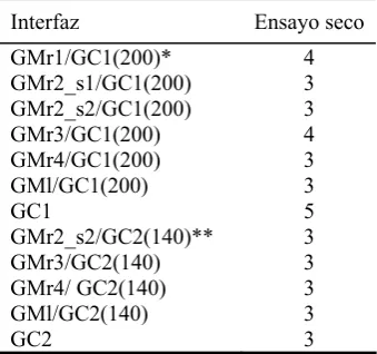
The conditions and velocities of the different tests are shown in Figure 5. This sketch presents the values of hydration time, consolidation time and horizontal displacement rate, depending on type of interface and test conditions: dry or wet. These values are the results of study and analysis of different research, Fox et al. (1998), Gilbert et al. (1996), Eid et al. (1999), Nye and Fox (2007), Pasqualini et al. (2002), Stark and Poeppel (1994), Sharma et al. (2007), Triplett and Fox (2001), Zornberg et al. (2005). Data of direct shear test is shown in Table 2.

Table 2. Summary of conditions test

Interface Size sample (mm)

Range normal stress (kPa)

Test condition

thydra. (h)

tconsol. (min)

Shear rate (mm/min)

GT/GM 300x285 14-450 wet 24/0 10 5

GC/GCL 300x285 100-500 dry 0/0 10 5

GCL/GM 300x285 100-500 wet 48/0 1440 0.055

Soil/GM 200x200 100-500 dry 0/0 10 1

The normal stress represents the normal load applied to the base lining system. The shearing was carried out until a horizontal displacement of 50 mm was achieved. The situation of the geosynthetics inside the machine is shown in Figure 5, as necessary devices. The test procedures were carried out in compliance with ASTM D5321-02 and included a specific methodology and the new geosynthetic fix system developed in this research. The readings during shearing were taken automatically by a computerized data logging system.

(34)

4. Analysis of results

Figure 10 and 11 show the direct shear test is repeated at different normal stress, the data is plotted, a trend is established, and the Coulomb failure criterion,

φ σ

τ =c_a + ⋅tan , is adjusted, where

τ

is the shear strength, ca is the adhesion, 

σ

is

the normal stress and

φ

 is the friction angle. The parameters ca and

φ

, are only useful

for the range of normal stress tested. Adhesion, ca must been considered as an

adjustment parameter without physical significance. It takes negative values when the slope of the failure line increases with the normal stress.

From the results, the strength behaviour was studied, as well as, analysing the developed interaction mecanism between tested materials.

Next, as a representative example of the research carried out, some interfaces, shown in Table 2, are briefly analysed: geotextile/geomembrane, geocomposite/GCL, GCL/geomembrane and soil/geomembrane. These tests are a small part of the investigation.

Direct shear test on geotextile/geomembrane

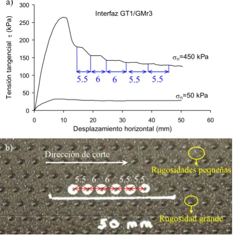
The shear stress versus horizontal displacement curves are illustrated in Figure 6. The peak shear stresses were mobilized at displacements of 2 mm to lower normal stress than 50 kPa, and between 7 mm and 12 mm to normal stress range 50-450 kPa. At low normal stress the shear stress reaches the peak and maintaining it until the end of the test. At normal stress higher than 50 kPa the curves after reaching the peak shear stress fall until they achieve residual value, showing strain-softening behaviour.

In this way, the interaction mechanism of the contact is different at low and high normal stress. This interface type shows two different mecanisms: hook and loop and frictional. At low normal stress the hook and loop and friction mecanism are small in superficial level and specific contacts. However, at high normal stress the geotextile becomes compressed and increasingly interbedded between the macroroughness of the contacting geomembrane resulting in matrix level frictional and hook and loop interactions.

(35)

Thesis summary 37

The samples were observed after testing, checking that geotextiles fibers were separated, stretched and oriented in shear direction, at normal stress higher than 50 kPa. This damage provides the strain-softening behaviour observed. Futhermore, at 450 kPa normal stress, some asperities of the geomembrane were damaged.

0 25 50 75 100 125 150 175 200 225 250 275

0.0 5.0 10.0 15.0 20.0 25.0 30.0 35.0 40.0 45.0 50.0 55.0

Horizontal displacement (mm)

S

h

e

a

r

st

r

ess

(k

P

a

)

ns = 14 kPa ns = 25 kPa ns = 50 kPa ns = 100 kPa ns = 300 kPa ns = 450 kPa

Figure 6. Shear stress-displacement curves for interface GT/GM

Direct shear test on drainage geocomposite/GCL

The shear stress versus horizontal displacement curves are illustrated in Figure 7. The maximum shear stresses were mobilized at displacements of 7.5-12 mm.

The GCL/drainage geocomposite interface shear strength behaviour, tested in dry conditions, is influenced by the thickness and stiffness of the geonet. In this way, the higher the thickness and stiffness the higher shear resistance, because the geonet embeds in the GCL.

In this case, the peak and residual friction angles and adhesion values were 26º, -21 kPa and 18º, -2 kPa respectively, as depicted in Figures 10 and 11. The failure plane of all tests is between the geocomposite and GCL.

(36)

Direct shear test on GCL/geomembrane

Figure 8 shows the results from wet conditions GCL/GM interface test. The peak shear stresses were mobilized at displacements of 6-7 mm. After that, the curve falls quickly to reach the residual value.

The GCL becomes compressed and interbedding between geomembrane texture causes geomembrane-GCL contact friction to be higher than internal GCL friction. In this case, the tests showed failure plane inside GCL, between woven geotextile and bentonite layer.

The shear resistances parameters obtained from lineal adjustment were: peak friction angle and adhesion values, 4º and 39 kPa, residual adhesion, 9 kPa as showed in Figures 10 and 11.

0 25 50 75

0.0 5.0 10.0 15.0 20.0 25.0 30.0 35.0 40.0 45.0 50.0 55.0

Sh

e

a

r

st

r

ess

(k

P

a

)

ns = 100 kPa ns = 300 kPa ns = 500 kPa

Figure 8. Shear stress-displacement curves for interface GCL/GM

Direct shear test on soil/geomembrane

Figure 9 presents shear stress versus horizontal displacement curves. These curves show strain softening behaviour. Firstly shear stress reaches a peak and then the curve falls to residual value. The peak shear stresses were mobilized at displacements of 6-7.5 mm. The peak and residual friction angles and adhesion values were 34º, 41 kPa and 23º, -28 kPa respectively as depicted in Figures 10 and 11.

The interaction mecanism are soil-geomembrane contact and internal soil friction. The higher the acumulated soil between asperities the higher the shear strength.

(37)

Thesis summary 39

came into contact with the gravel. It was observed that some soil stayed between the asperities as in Figure 12.

0 25 50 75 100 125 150 175 200 225 250 275 300

0.0 5.0 10.0 15.0 20.0 25.0 30.0 35.0 40.0 45.0 50.0 55.0

Sh ea r st r es s ( kP a )

ns = 100 kPa ns = 300 kPa ns = 500 kPa

Figure 9. Shear stress-displacement curves for interface soil/GM

0 25 50 75 100 125 150 175 200 225 250 275 300 325

0 25 50 75 100 125 150 175 200 225 250 275 300 325 350 375 400 425 450 475 500 525

Normal stress (kPa)

S h ea r s tre ss (k P a ) GT/GM GC/GCL GCL/GM Soil/GM

Figure 10. Peak failure envelopes

0 25 50 75 100 125 150 175 200 225 250 275 300

0 25 50 75 100 125 150 175 200 225 250 275 300 325 350 375 400 425 450 475 500 525

Normal stress (kPa)

S h ea r s tres s (k P a ) GT/GM GC/GCL GCL/GM Soil/GM

(38)

Figure 12. Contact between soil and texture geomembrane

5. Model and numerical analysis of the direct shear test

Frecuently, interface shear strength presents a non-linear behaviour. In this case, Coulomb parameters (ca, φ) are not much safer or realistic. For this reason, a new strength model and three-dimensional numerical analysis of the mechanical response of the textured geomembrane/nonwoven geotextile interface in direct shear were developed. The model was developed to simulate progressive failure of textured geomembrane/nonwoven geotextile interface, and it was used to investigate mechanisms of progressive interface failure and factors that control its significance.

Shear strength model

The shear strength model of textured geomembrane/nonwoven geotextile interface arose from the resemblances between the roughness rock joint and geomembrane/geotextile interface behaviour. Therefore, this model has been developed following the research of Barton (1973), Barton and Choubey (1977), Bandis et al. (1983), Barton et al. (1985), Stark et al. (1996), and the geosynthetic interface interaction mecanism from Hebeler et al. (2005). Achieving an equation of the following type:

⎥ ⎦ ⎤ ⎢ ⎣ ⎡ + ⎟⎟ ⎠ ⎞ ⎜⎜ ⎝ ⎛ ⋅ ⋅ = _r n n GCS I HL φ σ σ

τ tan log (1)

where

τ maximum shear stress (strength) of a

textured geomembrane/non-woven geotextile

n

σ normal stress

HL hook and loop coefficient I interbedding coefficient

GCS geotextile reference compression stress

r

φ residual friction angle

Shear direction

Soil

asperity

(39)

Thesis summary 41

Geotextile reference compression stress (GCS)

The geotextile compression stress (GCS) is a reference value for the normal stress on the geotextile which corresponds to a normal deformation of 0.8 for the geotextile (Figure 13). GCS controls the shear strength of the textured geomembrane/geotextile interface, which is influenced by the amount of interbedded, asperity and fibers damage. The GCS value is calculated from the relation between normal stress and vertical deformation of the geotextile. This relation is based on standard ISO 9863-1:2005 (procedure B). To measure compressibility and deduce GCS a uniaxial test system was used. The applied normal stresses varied from 2 to 35000 kPa. TheGCS values of tested geotextiles were: GT_nwnp_mf (nonwoven needle punched monofilament): 15000 kPa, GT_nwnp_st (nonwoven needle punched staple fibers): 4000 KPa and GT_nwhb_mf (nonwoven heat bonded monofilament): 35000 kPa.

0 10000 20000 30000 40000

0.1 0.2 0.3 0.4 0.5 0.6 0.7 0.8 0.9

Vertical deformation N o rm a l s tre ss (k P a )

Figura 13. Compressibility of GT_nwnp_mf

Hook and Loop (HL)

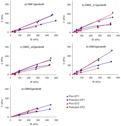
The hook and loop coefficient (HL) represents the engagement of the geotextile fibers (“loop” structure) by geomembrane roughness (“hook” material). To obtain the hook and loop value, HL, first the R value has to determined by back-analysing shear tests on the basis:

(40)

Next, R is plotted versus normal stress as shown in Fig. 14. From these graphs the hook and loop parameter (HL) is obtained for each geomembrane/geotextile interface. The

HL value is the intersection between the linear regession lines and the horizontal axis (R). The HL value depends mainly on the roughness of the geomembrane. For geomembranes with macrotexture > 1 mm (GMr3 and GMr2_s1), the HL value is between 4 and 8, and for geomembranes with macrotexture < 1 mm (GMr1, GMr2_s2 and GMr4), the HL values is between 2 and 4. This fact has a great influence on the peak shear strength value and the strain-softening behaviour.

Geomembranes macrotexture >1 mm

0 100 200 300 400 500

0 2 4 6 8 10 12 14 16 R N o rm a l s tre ss (k Pa ) GT_nwnp_mf/GMr2_s1 GT_nwnp_mf/GMr3 GT_nwnp_st/GMr2_s1 GT_nwnp_st/GMr3 GT_nwhb_mf/GMr2_s1 GT_nwhb_mf/GMr3

Geomembranes macrotexture < 1 mm

0 100 200 300 400 500

0 2 4 6 8 10

R N o rm a l st re ss (kP a ) GT_nwnp_mf/GMr1 GT_nwnp_mf/GMr4 GT_nwnp_st/GMr1 GT_nwnp_mf/GMr2_s2 GT_nwhb_mf/GMr1 GT_nwnp_st/GMr2_s2 GT_nwnp_st/GMr4 GT_nwhb_mf/GMr2_s2 GT_mwhb_mf/GMr4

Figura 14. R vs. normal stress from geomembranes with macrotexture>1 mm and

<1mm

Interbedding (I)

The interbedding coefficient (I) between the macrotextural features of geomembrane and geotextile. To obtain individual interbedding parameter as a function of normal stress was plotted I vs. R log

(

GCS σn

)

for different material combinations, where I

value is equal to HL

R _{. Next, linear relations were obtained by least squares fitting, as}

(41)

Thesis summary 43 HL M GCS GCS N I n n ⋅ − ⎟⎟ ⎠ ⎞ ⎜⎜ ⎝ ⎛ ⎟⎟ ⎠ ⎞ ⎜⎜ ⎝ ⎛ = σ σ log log (3) Interface: GT_nwnp_mf/geomembrane 0 0.5 1 1.5 2 2.5

0 2 4 6 8

R / log (GCS/σn)

Int er be ddi ng ( I) _GMr1 GMr2_s1 GMr2_s2 GMr3 GMr4

Figura 15. Interbedding for nonwoven geotextile/geomembrane interfaces

Numerical analysis using FLAC3D

To carry out numerical analysis the code FLAC3D was used. This code is a three-dimensional explicit finite-difference program to solve mechanical behaviour of a continous medium as it reaches equilibrium or steady flow.

Model setup

(42)

FLAC3D 3.00

Itasca Consulting Group, Inc. Minneapolis, MN USA Step 262 First Person Perspective 16:52:10 Tue Jun 10 2008 Eye Position: X: -4.612e-001 Y: -5.784e-001 Z: 3.114e-001

Eye Direction: X: 0.604 Y: 0.720 Z: -0.342 Eye Vertical: X: 0.220 Y: 0.262 Z: 0.940

Mag.: 0.8 Ang.: 22.500

Job Title: Direct Shear test between geotextile and geomembrane

Block Group top bot Axes Linestyle X Y Z Interface Locations Axes Linestyle X Y Z FLAC3D 3.00

Itasca Consulting Group, Inc. Minneapolis, MN USA Step 2161 Model Perspective 16:30:21 Fri Jul 11 2008 Center: X: 1.552e-001 Y: 1.486e-001 Z: -2.003e-002

Rotation: X: 20.000 Y: 0.000 Z: 50.000 Dist: 1.371e+000 Mag.: 0.96

Ang.: 22.500

Contour of SZZ Magfac = 1.000e+000

Gradient Calculation

-3.0555e+005 to -3.0000e+005 -3.0000e+005 to -2.8000e+005 -2.8000e+005 to -2.6000e+005 -2.6000e+005 to -2.4000e+005 -2.4000e+005 to -2.2000e+005 -2.2000e+005 to -2.0000e+005 -2.0000e+005 to -1.8000e+005 -1.8000e+005 to -1.7636e+005

Interval = 2.0e+004

Axes Linestyle

X Y

Z

a) b)

Figure 16. a) Interface between two sub-grids b) Initial conditions: application normal

stress

Modelling procedure

Figure 17 a) shows however the direct shear test is simulated by applying a horizontal velocity to the top sub-grid, to produce a shear displacement along the interface.

Figure 17 b) presents the shear stress-shear displacement curve. The loading is initially linear, and then becomes nonlinear as interface begins to fail until the peak shear strength, after that the shear strength decreases up to post-peak (residual) value. The plot also indicates whether stresses within a zone are currently on the yield surface (black points) or the zone has failed on the past (red points)

FLAC3D 3.00

Itasca Consulting Group, Inc. Minneapolis, MN USA Step 509621 Model Perspective 08:52:09 Wed Jun 11 2008 Center: X: 1.700e-001 Y: 1.602e-001 Z: 6.999e-004

Ang.: 22.500

Block Group top bot

Interface Locations

Displacement Maximum = 5.000e-002 Linestyle Axes

Linestyle Y X

Z

FLAC3D 3.00

Itasca Consulting Group, Inc. Minneapolis, MN USA Step 504270 Model Perspective 21:32:31 Wed Jul 16 2008 Center: X: 2.125e-001 Y: 1.577e-001 Z: 8.816e-002

Ang.: 22.500

Interface Shear Stress 0.0000e+000 to 2.0000e+004 2.0000e+004 to 4.0000e+004 4.0000e+004 to 6.0000e+004 6.0000e+004 to 8.0000e+004 8.0000e+004 to 1.0000e+005 1.0000e+005 to 1.2000e+005 1.2000e+005 to 1.2818e+005

Interval = 2.0e+004

Interface Shear Slip slipped now slipped in past Interface Locations History

1.0 2.0 3.0 4.0 x10^1 0.2 0.4 0.6 0.8 1.0 1.2 1.4 x10^2

4 sstav (FISH function) Linestyle 1.591e+000 <-> 1.494e+002 Vs.

FLAC3D 3.00

Itasca Consulting Group, Inc. Minneapolis, MN USA Step 509621 Model Perspective 08:52:09 Wed Jun 11 2008 Center: X: 1.700e-001 Y: 1.602e-001 Z: 6.999e-004

Ang.: 22.500

Block Group top bot

Interface Locations

Displacement Maximum = 5.000e-002 Linestyle Axes

Linestyle Y X

Z

FLAC3D 3.00

Itasca Consulting Group, Inc. Minneapolis, MN USA Step 504270 Model Perspective 21:32:31 Wed Jul 16 2008 Center: X: 2.125e-001 Y: 1.577e-001 Z: 8.816e-002

Ang.: 22.500

Interface Shear Stress 0.0000e+000 to 2.0000e+004 2.0000e+004 to 4.0000e+004 4.0000e+004 to 6.0000e+004 6.0000e+004 to 8.0000e+004 8.0000e+004 to 1.0000e+005 1.0000e+005 to 1.2000e+005 1.2000e+005 to 1.2818e+005

Interval = 2.0e+004

Interface Shear Slip slipped now slipped in past Interface Locations History

1.0 2.0 3.0 4.0 x10^1 0.2 0.4 0.6 0.8 1.0 1.2 1.4 x10^2

4 sstav (FISH function) Linestyle 1.591e+000 <-> 1.494e+002 Vs.

a) b)

(43)

Thesis summary 45

Analysis of results

Figure 18 shows examples of the shear stress-displacement data obtained from different geotextiles/geomembranes interfaces: GT_nwhb/GMr3, GT_nwnp_mf/GMr1 and GT_nwnp_st/GMr4. These interfaces were tested at different normal stress levels and compared with the numerical model (right diagram). Good agreement between the numerical model and the direct shear test is indicated.

GT_nwnp_mf/GMr1 25 50 100 300 450 0 50 100 150 200 250

0 5 10 15 20 25 30 35 40 45 50 Horizontal displacement (mm)

S hear st re ss ( kP a )

Flac model Direct shear test 300x300 mm

σn(kPa)

GT_nwhb_mf/GMr2_s2 25 kPa 50 kPa 100 kPa 300 kPa 450 kPa 0 50 100 150 200 250

S hear s tr es s ( kP a)

σn(kPa)

GT_nwnp_mf/GMr1 25 50 100 300 450 0 50 100 150 200 250

S hear st re ss ( kP a )

σn(kPa)

GT_nwhb_mf/GMr2_s2 25 kPa 50 kPa 100 kPa 300 kPa 450 kPa 0 50 100 150 200 250

S hear s tr es s ( kP a)

σn(kPa)

(44)

(45)

Presentación de la tesis 47

Presentación de la tesis

La presente tesis doctoral se divide en cuatro capítulos. Estos capítulos están precedidos por los siguientes elementos: lista de figuras, lista de tablas, notación empleada, el resumen de la tesis, en español e inglés y la presentación del documento.

Previamente se presenta una introducción de la situación medioambiental en materia de vertederos de residuos sólidos urbanos, así como la motivación y objetivos de la investigación.

El capítulo 1 es el estado del conocimiento, donde se repasa tipos y funciones de los diferentes geosintéticos, se cita diferentes tipos de roturas de vertederos, se revisa las investigaciones llevadas a cabo por diferentes autores para la realización del ensayo de corte directo de las interfaces geosintético/geosintético y suelo/geosintético, y se enumera los modelos de comportamiento de las juntas de roca, que son la base del modelo desarrollado de resistencia al corte de la interfaz geomembrana/geotextil.

El capítulo 2 presenta la metodología de ensayo de corte directo para las interfaces geosintético/geosintético y suelo/geosintético y obtención de los parámetros resistentes al corte.

El capítulo 3 presenta el análisis de los resultados de los ensayos de laboratorio de las diferentes interfaces ensayadas, y se describe el comportamiento resistente al deslizamiento de cada contacto.

El capítulo 4 desarrolla un modelo de comportamiento resistente al corte y el análisis numérico para la interfaz geomembrana rugosa/geotextil no tejido.

Finalmente se establecen las principales conclusiones que se derivan de esta tesis doctoral, recogiéndose así mismo, las futuras líneas de investigación que surgen de los estudios realizados.

(46)

Esquema de la metodología de la tesis doctoral Programa de ensayos corte directo 300x300 mm de las interfaces geosintético/geosintético y suelo/geosintético

Modelo

Formulación empírica

Modelo numérico Análisis por diferencias finitas

Conclusiones y futuras líneas de investigación

Metodología de ensayo Diseño caja de corte

Realización del programa de ensayos

Análisis de resultados

(47)

Introducción 49

Introducción

La Unión Europea es la segunda economía mundial tras los Estados Unidos. El crecimiento económico en el mundo desarrollado va asociado al uso intensivo de recursos.

La ampliación, los cambios demográficos y la globalización son factores impulsores de los cambios sociales en Europa. Uno de estos cambios es el aumento de las aglomeraciones urbanas, ya que los ciudadanos buscan una mejora de su calidad de vida y se trasladan allí donde las oportunidades laborales son mayores. Se estima que más del 80% de los europeos vivirán en áreas urbanas en el 2020. Por tanto la expansión urbana generará presión sobre la tierra, el transporte y el consumo. La mayoría de los nuevos hogares serán pequeños, reflejando los cambios sociales y el estilo de vida tal como el creciente número de familias de pocos miembros o personas que viven solas.

La gestión del medio ambiente de Europa y de su capital natural es importante para garantizar el capital social y económico a largo plazo. Uno de los aspectos de mayor relevancia a gestionar, junto al consumo de energía y a los sucesos catastróficos relacionados con el clima y el tiempo, es la generación de residuos cada vez mayor debido al crecimiento económico y a los patrones de consumo (por ejemplo el aumento del consumo de productos envasados, cuyos envases se suman al crecimiento de residuos de embalaje provenientes de los hogares). Las opciones de tratamiento de los residuos preocupan por sus impactos en el medio ambiente, y la salud de las personas. Decidir la ubicación de las incineradoras es un asunto controvertido en muchos países, y la opción de los vertederos a menudo se ve limitada por el espacio y la contestación social, además de por el temor a la contaminación del suelo y de las aguas subterráneas.

En las últimas décadas, España ha seguido la estela del crecimiento económico europeo como una de las economías más dinámicas dentro de Europa. Este desarrollo económico ha supuesto una mejora de la calidad de vida de la mayoría de los españoles, aunque el coste medio ambiental es muy elevado, sobre todo a largo plazo. Según el Ministerio de Medio Ambiente, actualmente en España:

(48)

- crece la demanda de transporte de mercancías y de pasajeros por encima de la

media europea

- existen cada vez más residuos

- subsisten las amenazas sobre ecosistemas terrestres y marítimos - disminuye la capacidad de pesca

- urge una mejor eficiencia en el uso del agua y en el de la energía

- hay una mala utilización y abuso de fertilizantes sintéticos y plaguicidas.

(49)

Introducción 51

Uno de los problemas más importantes relacionados con el medio ambiente es la generación creciente y constante de residuos urbanos:

GENERACIÓN DE RESIDUOS URBANOS

España

UE-15

500 550 600 650 700

1995 1996 1997 1998 1999 2000 2001 2002 2003 2004 2005 2006 2007

Fuente: EUROSTAT

kg

/h

ab.

a

ñ

(50)

Residuos urbanos recogidos 0 40 80 120 160 200 240 Ale m an ia E sp aña Fra nc ia Ita lia Re in o Un id o UE-1 5 Residu os u rb ano s ( m ill. ton s)

Residuos urbanos vertidos

0 20 40 60 80 100 120 Al em a ni a Esp añ a Fr a nc ia Ita lia Re in o Un id o UE -1 5 Residu os u rb ano s ( m ill. ton s)

1996 2000 2004

Residuos urbanos incinerados

0 10 20 30 40 50 A lem ani a

España Franc

ia Ita lia R e ino U ni do UE-1 5 R es iduos u rbano s (m ill. t o n s) Fuente: EUROSTAT

La Comunidad Europea adoptó la Directiva 91/156/CEE y la Directiva 1999/31/CE, para establecer las premisas comunitarias sobre la gestión de residuos y vertidos, respectivamente, que deben cumplir todos los Estados miembros. La adaptación de la Directiva 91/156/CEE al Estado español dio lugar a la Ley 10/1998 que establece las normas para la gestión de residuos, siendo complementada por el Real Decreto 1481/2001 (adaptación de la Directiva 1999/31/CE), que constituye un reglamento para la eliminación de residuos mediante su depósito en vertederos con el objeto de prevenir los efectos ambientales negativos del vertido. Dentro de la Ley 10/1998 y el RD 1481/2001 se definen los distintos tipos de residuos:

- «Residuos urbanos o municipales»: los generados en los domicilios particulares,

comercios, oficinas y servicios, residuos procedentes de la limpieza de las vías públicas, zonas verdes, áreas recreativas y playas, animales domésticos muertos, muebles, enseres y vehículos abandonados, residuos y escombros procedentes de obras menores de construcción y reparación domiciliaria

- «Residuos peligrosos»: objetos, sustancias y preparados que presenten o puedan

presentar riesgos inmediatos o diferidos para la salud humana y el medio ambiente. El RD 952/1997 contiene la lista de residuos peligrosos.

- «Residuos no peligrosos»: los residuos no incluidos en la lista de residuos

tóxicos y peligrosos del RD 952/1997.

- «Residuos inertes»: aquellos residuos no peligrosos que no experimentan

transformaciones físicas, químicas o biológicas significativas.

(51)

Introducción 53

viene establecida en el Plan Nacional de Residuos Urbanos (2000-2006), elaborado a partir de la Ley 10/1998, donde se fijan las siguientes opciones de gestión:

- Reciclado - Compostaje - Incineración

- Eliminación en vertedero

En los gráficos y tabla siguientes se resume la situación de la gestión de los residuos urbanos según el Plan.

SITUACIÓN AÑO 1996

Vertido 70% Incineración 4% Reciclaje 12% Compostaje 14%

Fuente: Plan Nacional de residuos urbanos (2000-2006) y Borrador del Plan Nacional Integrado de Residuos (Octubre 2008)

Año 1996 2004 2006

Población (hab.) 39.669.394 43.197.684 45.200.737

Generación RU (ton) 17.175.186 22.807.748 24.078.306

Tasa generación RU (Kg./hab.día) 1.2 1.5 2

Producción RU (Kg./hab.año) 440 540 730

Fuente: MMA y Eurostat

En los gráficos se observa que más de la mitad de los residuos urbanos son depositados en vertederos.

En el pasado reciente, los vertederos eran básicamente zonas relativamente apartadas del centro de las poblaciones donde, sobre el terreno, se depositaba la basura para que se pudriera.

Este sistema es un riesgo potencial para el medio ambiente puesto que no impiden que los contaminantes (como metales pesados y toxinas) se filtren a través del terreno y contaminen las aguas subterráneas.

Si no se establecen los medios oportunos, los vertederos pueden contaminar:

- El aire, mediante emisiones de CO2 (dióxido de carbono) y CH4 (metano);