On Power Law Relationships of IDR Changes-Edición Única

(1)

Instituto Tecnológico y de Estudios Superiores de Monterrey Campus Monterrey

Monterrey, Nuevo León a

en los sucesivo LA OBRA, en virtud de lo cual autorizo a el Instituto Tecnológico

y de Estudios Superiores de Monterrey (EL INSTITUTO) para que efectúe la divulgación, publicación, comunicación pública, distribución y reproducción, así como la digitalización de la misma, con fines académicos o propios al objeto de EL INSTITUTO.

El Instituto se compromete a respetar en todo momento mi autoría y a

otorgarme el crédito correspondiente en todas las actividades mencionadas anteriormente de la obra.

De la misma manera, desligo de toda responsabilidad a EL INSTITUTO por cualquier violación a los derechos de autor y propiedad intelectual que cometa el suscrito frente a terceros.

Nombre y Firma AUTOR (A)

de 200

Lic. Arturo Azuara Flores:

Director de Asesoría Legal del Sistema

Por medio de la presente hago constar que soy autor y titular de la obra

(2)

On Power Law Relationships of IDR Changes-Edición Única

Title On Power Law Relationships of IDR Changes-Edición Única

Authors Jesus Rubén Gómez Zamorano Affiliation ITESM

Issue Date 2006-12-01 Item type Tesis

Rights Open Access

Downloaded 19-Jan-2017 10:22:26

(3)

INSTITUTO TECNOLÓGICO Y DE ESTUDIOS

SUPERIORES DE MONTERREY

CAMPUS MONTERREY

PROGRAMA DE GRADUADOS EN TECNOLOGÍAS DE

INFORMACIÓN Y ELECTRÓNICA

On Power Law Relationships of IDR Changes

THESIS

Presented as a partial fulfillment of the requirements for the degree of

Master of Science in Electronic Engineering

Major in Telecommunications

Jesús Rubén Gómez Zamorano

(4)

INSTITUTO TECNOLÓGICO DE ESTUDIOS SUPERIORES DE MONTERREY

DIVISIÓN DE TECNOLOGÍAS DE INFORMACIÓN Y ELECTRÓNICA

PROGRAMA DE GRADUADOS EN TECNOLOGÍAS DE INFORMACIÓN Y ELECTRÓNICA

The members of the thesis committee recommended the acceptance of the thesis of Jesús Rubén Gómez Zamorano as a partial fulfillment of the requirements for the degree of

Master of Science in:

Electronic Engineering

Major in Telecommunications

Thesis Committee:

______________________________

César Vargas Rosales, Ph.D. Advisor

______________________________

Artemio Aguilar Coutiño, M.Sc. Synodal

______________________________

Carlos Mex Perera, Ph.D. Synodal

_________________________________________

Graciano Dieck Assad, Ph.D. Director of the Graduate Program

(5)

On Power Law Relationships of IDR Changes

Jesús Rubén Gómez Zamorano

THESIS

Presented as a partial fulfillment of the requirements for the degree of

Master of Science in Electronic Engineering

Major in Telecommunications

INSTITUTO TECNOLÓGICO Y DE ESTUDIOS

SUPERIORES DE MONTERREY

(6)

To my parents, to whom I owe everything I am and everything I’ll ever be.

(7)

Acknowledgments

To my family, for supporting me in every endeavor I’ve started.

To my friends, for standing by my side through thick and thin.

To my thesis advisor, for his guidance through the completion of this work.

(8)

Abstract

In this work data obtained from an interdomain routing protocol (IDR) is used to create a topology map of the network in the interdomain level. With the statistical description of the obtained topology, power law relationships are observed for the times between the changes in the number of routes in interdomain level links. These power law relationships are explained in terms of the power law relationships observed in the interdomain level topology. With this new information, the scalability issues (i.e. Internet growth) and security proposals for interdomain routing can be further analyzed with a different scope.

(9)

List of Graphics

Figure 2.1 Graphical depiction of hierarchical routing 8

Figure 2.2 Stub AS example 8

Figure 2.3 Multihomed non-transit AS example 9 Figure 2.4 Multihomed transit AS example 10 Figure 2.5 BGP neighbor negotiation 12 Figure 2.6 BGP routing process 13 Figure 2.7BGP Routing Information Bases (RIBs) 14 Figure 2.8 Network topology example 18 Figure 2.9 LinkRank graph example 20 Figure 3.1 Flow chart for the topology maps creation process 24 Figure 3.2 Region graph example 26 Figure 3.3 Resulting graph from the BGP graphing algorithm 27 Figure 3.4 Flow chart for the statistical analysis of LinkRank Data 28 Figure 3.5 Original data versus different models for the 701-7018 link 29 Figure 3.6 Log-log plot of original data versus different models for the 701-7018 link 30 Figure 3.7 Original data versus different models for the 701-1239 link 31 Figure 3.8 Log-log plot of original data versus different models for the 701-1239 link 32 Figure 3.9 Two interdomain nodes with high degree 33 Figure 3.10 Original data versus different models for the 3130-1239 link 34

Figure 3.11 Log-log plot of original data versus different models for the 3130-1239 link 35

Figure 3.12 Link between a high degree node and a low degree node 36 Figure 3.13 Original data versus different models for the 3130-7575 link 37

Figure 3.14 Log-log plot of original data versus different models for the 3130-7575 link 37

(12)

List of Tables

(13)

Chapter 1 Introduction

The Internet has greatly evolved from a small and controlled network serving only a few users in the late 1970s (ARPANET) to an immense multilayered mesh of millions of terminals, routers, and many other components that interact with each other in a highly complex fashion.

The evolution has been incredible fast in an unregulated and open environment in comparison with other telecommunication systems which had a more controlled evolution (like the telephone), [1]. This lack of control and regulation has made the connectivity mapping and performance analysis of Internet a particularly complex task.

Also, Internet growth has become a major issue; many works express a concern on the plausibility of a collapse of the current system, [2]. Most of the stress in Internet is concentrated on the routing protocols, in particular interdomain routing, [3], [4].

A similar concern arose in 1993-1994 when the IP address space had to be reorganized in order to prevent a collapse in the address allocation. For this issue Classless Interdomain Routing (CIDR) was created. In the present day a similar problem occurs in interdomain routing where the announcement of many small networks, particularly for multihoming, is greatly increasing the length of the routing tables and the implementation of IPv6 will only aggravate the problem, [3].

It is well known that BGP’s work depend primarily on the topology of the network on which it is implemented, [3], [12]. The connectivity and reachability provided depend on it, but also, the topology is used to communicate all the different routing messages needed to maintain and update such connectivity. Even though reachability also depends on administration constraints (the human factor), all changes affect how each node perceives the connectivity and, in the end, the topology of the network.

The Border Gateway Protocol (BGP) was developed during a time when Internet didn't have the security risks of today. Therefore, it was developed thinking in its functionality rather than its security [5], [6].

(14)

important research issue. However, it is a difficult task for various reasons, [7]. In particular the search of a starting point and the constraints many administrators put on topology information (due to competitive issues). Comprehending the topology and its nodes interaction is the key to understand present behavior and predict future issues; scalability being one of those.

Generally the scalability problems in routing systems in the past have been “solved” using patches in the current configurations (i.e. CIDR). Some propose the same for the next scalability issue, while others proposed a totally different scope in the form of a new routing paradigm, [8]. Although neither one is in the scope of this work, it is useful to notice that a measurement of how well they fare in real practice is necessary, and that is what this work proposes.

This works proposes a measurement of a node, an Autonomous System (AS) in the IDR case, importance, based on a group of simple metrics obtained from real routing data.

A node importance will be a function of its neighbor connectivity, external connectivity

and outbound reachability. The neighbor connectivity refers to how many nodes are

directly connected; external connectivity refers to how far is the nearest non-group node (or nodes) and outbound reachability is a measurement of how reliable the outbound links of a node are.

Neighbor connectivity and external connectivity are measured using data obtained from public domain BGP dumps (RIS RIPE) and processed utilizing a java package known as JUNG (Java Universal Network Graph Framework). Also, connectivity maps are obtained from this data. These maps feature AS connectivity in a region (being a country the smallest region) and its connectivity to the exterior.

Outbound reachability is measured utilizing LinkRank [9] data obtained from Oregon University and processed in java and MySQL. The statistical analysis of this data will give an overlook of the real behavior of BGP links.

1.1 Problem Definition

(15)

The unregulated and open environment of Internet makes scalability measurements a difficult task, one that the creators did not foresee, yet a very important one. Therefore, these measurements must be done indirectly observing related variables. Network topology and routing information are particularly important.

Indirect methods must be used to obtain topology descriptions from measurable data. An algorithm is defined in this work for the creation of region oriented topology maps. Being region oriented not only for scale and data processing issues, but also for the need of obtaining region focused behavior.

From the topology description routing parameters that inherently depend on it can be measured. Obtaining a relationship between the topology and the routing parameters we can gain future insight of the network behavior.

With measurements of the past and current behavior of the Internet topology and the relations it creates (observed in the routing information) models can be created to predict future behavior and relate it to the scaling capabilities of the network.

Given the current performance of the networks, future performance could be measured and the scalability problems could be adverted. Also, predicting the magnitude of the problem a profit-cost analysis could be done to compare different approaches, mainly the feasibility of continuing doing patches, or the necessity of doing a complete paradigm shift.

1.2 Hypothesis

The statistical behavior of the time between the changes in the number of routes in an interdomain level link depends on the statistical description of the laying topology. Thus, statistical characterization will provide the behavior of the frequency at which the number of routes that traverse such link change and its explanation and significance from a topological point of view.

1.3 Objectives

We divide the main objectives of this thesis in four points as follows:

a) Obtain a connectivity map that shows the topology description for the interdomain level routing from real routing data of the utilized interdomain routing protocol.

(16)

c) Find a relationship between the statistical topology model of the interdomain architecture and the statistical behavior model for the times between the changes in the number of routes in an interdomain level link.

d) Observe the implications on scalability issues analysis and interdomain routing security proposals of the behavior model of the times between the changes in the number of routes in an interdomain level link previously presented for different node configurations.

1.4 Final Product

Topology maps for the interdomain level architecture from real routing data that show both the outbound and inbound connectivity for a defined region. For this product several subproducts will be obtained: a program that creates topology maps from interdomain routing data, an algorithm to create region oriented connectivity maps and a database with relevant data for all the assigned AS numbers.

A power law behavior model for the times between the changes in the number of routes in an interdomain level link is presented as a result in this work. This power law relationship is different from the ones seen in related works such as [26] and [28]. However, it is also related to the laying topology as the ones shown in those works, and consequentially it is also related to those power law relationships.

1.5 Contributions

This work uses some data and tools already available, but presents several contributions derived from them. A list follows:

• A Java based program that collects name and country of origin of all the

registered Autonomous Systems. Used for the topology maps in Chapter 3.

• A database containing the data collected from that program. Used for the topology maps in Chapter 3.

• A Java program that processes BGP dumps in ASCII format to create a MySQL

database. Used for the topology maps in Chapter 3.

• An algorithm for creating region oriented BGP topology graphics. Explained in

Chapter 3.

(17)

• A Java program that processes LinkRank data and creates a MySQL database containing the changes and the time of the changes. Used for the analysis of LinkRank data in Chapter 3.

• Analysis of the data contained in the previous database, comparing the results with various models. Used for the graphics of the frequency of the time between the changes in routes between interdomain nodes in Chapter 3.

• A power law relationship obtained from that analysis for different node configurations (high degree with high degree, low degree with high degree and low degree with low degree connections).

• An explanation of the causes of the observed power law relationships.

1.6 Summary

Chapter 2 contains the necessary background to understand the work proposed here. Routing principles in general and for interdomain routing (specifically the BGP protocol) are reviewed. Other topics include Internet Organization, the concept of Internet tomography, power law relationships in Internet Topology and the tool LinkRank for route change analysis.

Chapter 3 contains the methodology and results of the topology creation algorithm and the analysis of the times between the changes in the number of routes in an interdomain level link. Power law behavior is observed for the latter.

(18)

Chapter 2 Background

In this section some relevant principles and concepts are explained for the better understanding of this work. This background represents the bases in which this work is built over.

2.1 Routing Principles

The packet transfer from a source to a destination requires a route to follow. The set of rules used by the network layer to choose between different routes is called the routing protocol.

At heart of any routing protocol is the routing algorithm, which finds, given a set of routers with links connecting them, a “good” path from source to destination.

Typically, a “good” path is one that has “least cost”. The definitions of “good” path and “least cost” depend on the used algorithm and protocol and on the network characteristics. Cost can be related to many measurements, either natural to the network characteristics (such as length of the path, number of hops, speed of the link) or user created (monetary cost of the path, business agreements between peers). However, in real practice, concerns such as policy issues also come into play, [10].

The problem of finding the least-cost path from a source to a destination requires identifying a series of links such that:

• The first link in the path is connected to the source • The last link in the path is connected to the destination

• For all i, the i and (i-1)st link in the path are connected to the same node

• For the least-cost path, the sum of the cost of the links on the path is the

minimum over all possible paths between the source and the destination. If all link costs are the same, the least-cost path is also the shortest path.

Now, when a policy has been defined to use costs to determine a good path, the routing algorithms carry out calculations with this policy to obtain the least cost path. This helps us to classify the routing algorithms in global and decentralized:

• A global routing algorithm computes the least-cost path between a source and

(19)

Algorithms with global state information are known as link state algorithms.

• A decentralized routing algorithm calculates the least-cost path in an iterative,

distributed manner. No node has complete information about the costs of all network links. Instead, each node begins with only the knowledge of the costs of its own directly attached links (i.e., the incident links to the node). One example is the distance vector algorithm, in which each node only knows the neighbor to which it should forward a packet in order to reach a given destination.

An alternate classification of routing algorithms does not depend on the amount of information nor on the fashion on which the calculations are executed. A second broad way to classify routing algorithms is according to whether they are static or dynamic. In static algorithms the routes change very slowly over time, often as a result of human intervention. In dynamic algorithms the routing paths changes as the loads or topology of the network changes, [10].

Only two types of routing algorithms are typically used in the Internet: a dynamic global link state algorithm and a dynamic decentralized distance vector algorithm.

2.1.1 Hierarchical Routing

In practice, the network can't be viewed simply as a collection of interconnected routers at least for two reasons, [11]:

• Scale. The large number of routers makes the overhead involved in computing,

storing, and communicating the routing table information prohibitive. The link state information of an algorithm of that size would leave no bandwidth left for sending data packets. A distance vector of that many nodes would never converge.

• Administrative autonomy. For many organizations is desirable to run they

routers as they please, or to hide certain internal organization information to the outside.

Therefore, routers are aggregated into regions known as autonomous systems (AS). Routers within the same AS run the same routing algorithm and have information about each other. The AS need to be interconnected, thus one or more routers in an AS will have to route packets within the AS and to the outside. That router is called a gateway router. The routing process between AS is know as interdomain routing, [10].

(20)

[image:20.612.133.481.76.252.2]

Figure 2.1 Graphical depiction of hierarchical routing

Autonomous systems are classified according to its network configuration.

2.1.1.1 Stub AS

An AS is considered a stub AS if it only has one exit point to communicate with networks outside its domain. They are also known as single-homed from its provider.

Figure 2.2 Stub AS example

A single-homed AS doesn’t need to learn Internet routes from its provider because it only has one exit, therefore all Internet traffic uses the default route to the provider.

[image:20.612.120.497.379.593.2]

(21)

2.1.1.2 Multihomed Non-transit AS

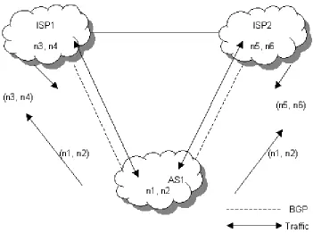
[image:21.612.132.483.182.443.2]

An AS is multihomed if it has more than one exit to the exterior. An AS can be multihomed from one or various providers. The nontransit property means that traffic cannot go through it.

Figure 2.3 Multihomed non-transit AS example

A nontransit AS will only announce its own routes and will not propagate the routes it learned from other AS. This assures that the traffic for any destination that doesn’t belong to the AS will not be directed to it. In the figure it can be seen that AS1 learns routes n3 and n4 from ISP1 and routes n5 and n6 from IPS2, but it only propagates its own routes: n1 and n2.

Multihomed nontransit AS’s do not need to run BGP with its providers, although it is recommended and, most of the time, required by them.

2.1.1.3 Multihomed Transit AS

A multihomed transit AS has various connections with the exterior and can be used to propagate traffic from other AS.

(22)

connections between routers from different AS are known as external BGP (EBGP). The

routers running IBGP are known as transit routers when they carry the traffic that goes through the AS.

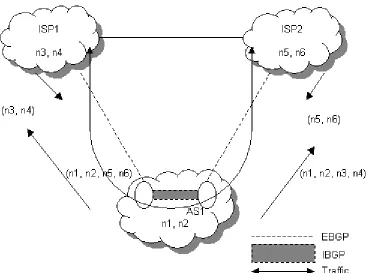
[image:22.612.123.490.166.439.2]

The utilization of BGP-4 is recommended for multihomed transit AS for its connections with other AS and to protect its non transit routers from the Internet routes.

Figure 2.4 Multihomed transit AS example

In Figure 2.4, AS1 works as a multihomed transit AS. It learns routes n3 and n4 from ISP1 and routes n5 and n6 from ISP2, and it announces everything it learns to its neighbors. Therefore, ISP1 uses it as a transit AS to reach n5 and n6 in ISP2, and ISP2 does the same thing to reach n3 and n4 in ISP1.

2.1.1.4 Routing Between Autonomous Systems

BGP-4, specified in RFC 1771, [13], is the standard interdomain routing protocol. In the wide sense, BGP can be considered as part of the distance vector protocols family, however is more properly characterized as a path vector protocol (PV).

In a classic distance vector protocol, all the information about the route to a destination is concentrated in the metric value. This is insufficient for fast loop resolution.

(23)

doesn't require that all relays use the same metrics, on the contrary, they are allowed to make arbitrary choices. Loops will be avoided if they update the path vectors according to the results of these choices.

The drawback is obvious: the increment on the routing messages size and the memory used to run the protocol, [12].

2.1.2 The BGP Protocol

As stated before, BGP is a PV protocol. It uses TCP as its transport protocol (via port 179). Therefore, all transport reliability is taken care by TCP.

Routers that run a BGP routing process are often referred to as BGP speakers. Two BGP speakers that form a TCP connection between one another to exchange route information are referred to as neighbors or peers.

2.1.2.1 BGP neighbor negotiation

Neighbor negotiation is based on the successful completion of a TCP transport connection, the successful processing of the OPEN message, and periodic detection of the UPDATE or KEEPALIVE messages.

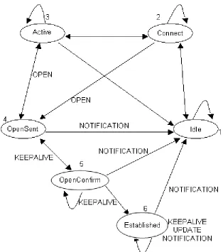
The BGP negotiation proceeds through different states before the connection is fully established. These are the key states, [11]:

1. Idle. BGP is waiting for a Start event, which is initiated by an operator or the

BGP system. After that event, BGP initializes its resources, resets a ConnectRetry timer, initiates a TCP connection, and starts listening for a connection from a remote peer. Connect.

2. Connect. BGP is waiting for the completion of the TCP connection. If

successful, transitions to OpenSent. If unsuccessful, transitions to Active. If the ConnectRetry timer expires it returns to the Connect state.

3. Active. BGP tries to acquire a peer by initiating a TCP connection. If

successful, transitions to OpenSent. If the ConnectRetry timer expires it returns to the Connect state. In general, a neighbor state that is oscillating between Connect and Active indicates that something is wrong with the TCP connection.

4. OpenSent. BGP is waiting for an OPEN message from its peer. In case of

errors, sends a NOTIFICATION message and returns to Idle. If there are no errors, BGP starts sending KEEPALIVE messages and resets the KEEPALIVE timer.

5. OpenConfirm. BGP waits for a KEEPALIVE message. If received goes to

(24)

[image:24.612.151.465.70.425.2]

Figure 2.5 BGP neighbor negotiation

2.1.2.2 BGP Messages

The NOTIFICATION message contains an error code, an error subcode and a data field. The error code indicates the type of notification, the error subcode provides more information and the data field contains data relevant to the error.

The KEEPALIVE messages are periodic and are exchanged between peers to determine reachability.

The UPDATE message is the core of the BGP protocol. It contains the routing updates that are the necessary information that BGP uses to construct a loop-free picture of the network. Its basic blocks are the Network Layer Reachability Information (NLRI), Path attributes and Unfeasible routes.

(25)

The path attributes are a set of parameters used to keep track of route specific information such as path information, degree of preference, NEXT_HOP, and aggregation information.

Path attributes fall into four categories: well-know mandatory, well-know discretionary, optional transitive, and optional nontransitive, [11].

2.1.2.3 The Routing Process

BGP is a fairly simple protocol. Routes are exchanged between peers by UPDATE messages. BGP routers receive those, run some policies or filters on them and then pass the routes to other BGP peers. BGP picks the best route and sends it. A BGP router can pass along EBGP routes from peers, IBGP routes from route reflector clients or advertise internal networks from its own AS. Valid local routes and the best routes received from peers are then installed in the IP routing table, which is the final routing decision and is used to populate the forwarding table.

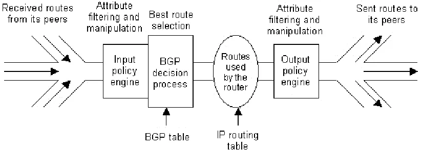
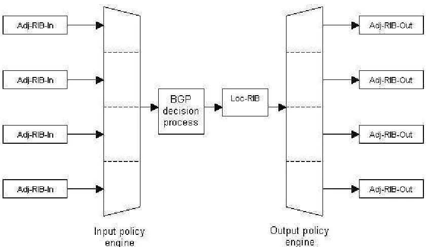
A model of the BGP process would involve the following components:

• A pool of routes that the router receives from its peers

• An Input Policy Engine that can filter the routes or manipulate their attributes • A decision process that decides which routes the router itself will use

• A pool of routes that the router itself uses

• An Output Policy Engine that can filter the routes or manipulate their

attributes

• A pool of routes that the router advertises to other peers

[image:25.612.97.510.477.624.2]

Figure 2.6 illustrates this model:

Figure 2.6 BGP routing process

2.1.2.4 BGP Routes: Advertisement and Storage

(26)

For purposes of this protocol a route is defined as a unit of information that pairs a destination with the attributes of a path to that destination:

• Routes are advertised between a pair of BGP speakers in UPDATE messages. The destination are the systems whose IP addresses are reported in the Network Layer Reachability Information (NLRI) field, and the path is the information reported in the path attributes fields of the same UPDATE message.

• Routes are stored in the Routing Information Bases (RIBs): namely, the

Adj-RIBs-In, the Loc-RIB, and the Adj-RIBs-Out. Routes that will be advertised to other BGP speakers must be present in the Adj-RIB-Out; routes that will be used by the local BGP speaker must be present in the Loc-RIB, and the next hop for each of these routes must be present in the local BGP speaker's forwarding information base; and routes that are received from other BGP speakers are present in the Adj-RIBs-In.

If a BGP speaker chooses to advertise the route, it may add to or modify the path attributes of the route before advertising it to a peer.

[image:26.612.88.512.405.649.2]

Figure 2.7 shows this structure:

(27)

Although in the figure there's a distinction between RIBs-In, Loc-RIB, and Adj-RIBs-Out in reality, most implementations store one copy of the information with pointers in order to conserve memory, [11].

2.1.2.5 BGP Decision Process Summary

BGP bases its decisions on the attribute values. The following process summarizes how BGP selects the best route:

1. If the next hop is unreachable, the route is ignored.

2. Prefer the path with the largest weight (Weight is a Cisco propietary parameter, local to the router)

3. If the weights are the same, prefer the route with the largest local preference value.

4. If there are no locally originated routes and the local preference is the same, prefer the route with the shortest AS_PATH

5. If the AS_PATH length is the same, prefer the route with the lowest origin type (where IGP is lower that EGP which is lower than INCOMPLETE). 6. If the origin type is the same, prefer the route with the lower MED value if the

routes where received from the same AS.

7. If the routes have the same MED value, prefer EBGP paths to IBGP paths. 8. If all the preceding scenarios are identical, prefer the route that can be reached

via the closest IGP neighbor.

9. If the internal path is the same, the BGP_ROUTER_ID will be a tiebreaker. Prefer the route coming from the BGP router with the lowest RID.

2.1.2.6 The Security Issue: Analysis of Related Work

There are many different approaches to BGP security, and each one has measured its results in some way trying to prove the effectiveness of their methods, nevertheless, they haven't done it using a mathematical framework.

The analysis done by S-BGP is based on NAPs statistics about the number of UPDATES created and the load increase that their add-ons create (PKIs and their new parameters). In his first analysis, [14], they estimated an UPDATE peak of 10 times the average load, in a more recent study, [15], it was observed that it could reach up to 200 times the average. It clearly can be seen that their methods could create a big increment in the system load and they'll need external NVRAM for the routers (it's stated the storage of databases up to 85 Mb in size that grow with time) and better processors, a pretty unreal supposition.

(28)

The protocol proposed by Cisco, soBGP, [16], supposes a lower load to the system and the update would only be at software level. However, it states the necessity of a trust network. Their publications don't show too much about the performed analysis, although it's compared with similar protocols and, analyzing the same parameters, highlights its advantages on processing costs and consumed bandwidth, and its easy deployment. But it isn't as safe as others (for example, it doesn't protect against changes during the transit of the UPDATE message) and it can affect convergence, [16].

One of the deepest analyses on security can be found on the Secure Path Vector proposal, [17]. It states the security measure as the probability that an attack could create false signatures, according to a system of their own. The probability of this happening is of 2²² at most, because the probability of a false signature creation is of 2¹¹ and at least two of them need to be created (taking them as independent events). Their model is only based on the number of ASN and the public and private keys need to be created. Under this supposition they calculate a computational cost and compare it against the one from S-BGP, being SPV a lot faster (up to 22 times faster). However, the protocol also needs hardware accelerators (but they argue a minor cost than S-BGP). In fact the test is done with PIII 1 Ghz processors.

Also, they don’t show in their graphs that their system provokes a header increment of 2.731 times and they don't analyze the effect of this on the system.

The other security proposals seek the creation of external networks or using other existing networks (like DNS) to support the BGP security. Therefore, they don't propose changes to the actual BGP structure, but they do affect its performance due the necessity of consulting external databases to evaluate the reliability of an announced route.

There are many works that propose the creation of BGP models, with diverse motivations. However, even if they seek to evaluate the performance under normal conditions, under pressure, under attacks, etc. The finality is always the same: anticipate the system reaction before doing a practical implementation. The operators need to do changes constantly to maintain a good performance. However, due to the distributive nature of the BGP route selection, the indirect control from configurable policies and the influence from complex interactions between other IDR protocols, the operators can't predict how a particular BGP configuration will work in practice, [18].

Nick Feamster’s article “A Model of BGP Routing for Network Enngineering”, [18], is a good reference point. It deals with the different characteristics of the BGP protocol operation, the problems it faces and some imposed constraints. It proposes an algorithm that explains the BGP route selection process. That differs from this works proposal. Also, it doesn't states any security measures.

(29)

comparing the mistakes done on the route selection. On a related work, Feamster proposes the separation of the interdomain routing from the IP routers, [19], to boost its performance.

Other related works proposed the creation of IGP emulators and a BGP convergence model, [20], [21]. This work doesn't state the creation of emulators, nor algorithms, but of a mathematical model, therefore, differing from other works. However, they can serve as a base considering the BGP protocol characteristics that they used to build their models.

2.2 Internet Organization

The Internet is a loosely-organized collaboration of autonomous and interconnected networks that supports host to host communication. Participation in the Internet depends on the voluntary adherence to Internet Standards.

2.2.1 Administration

The IANA (Internet Assigned Numbers Authority) has the responsibility of managing IP addresses and domain names at upper levels. This responsibility is delegated globally to the following bodies:

• RIPE NCC (Réseux IP Européens Network Coordination Center)

• ARIN (American Registry for Internet Numbers)

• APNIC (Asia Pacific Network Information Center)

• LACNIC (Latin America and Caribbean IP address Regional Registry)

• AfriNIC (African Regional Registry for Internet Number Resources)

They, also, delegate this responsibility to regional bodies in many countries.

2.2.2 Internet Operations

The IEPG (Internet Engineering Planning Group) coordinates worldwide Internet operations. It helps ISPs to interoperate within the global Internet. At global level this responsibility is delegated to:

• ARIN

• NANOG (North American Network Operators Group): an educational and

(30)

information related to backbone/enterprise networking technologies and operational practices.

• EOF (European Operators Forum Working Group): deals with operational

issues in Europe, such as new backbones and Internet Exchange Points.

• APNG (Asia Pacific Networking Group): promotes the Internet and coordination of network connectivity in the Asia Pacific region.

2.2.3 Internet Security

Internet network security is significantly facilitated by a number of Computer Emergency Response Teams (CERTs) in eight countries and within a number of service provider operations and private networks. They were formed to continually monitor the network for security incidents, serve as a repository for information about such incidents, and develop responsive advisories. The CERTs are coordinated by the Forum of Incident Response and Security Teams (FIRST).

2.3 Internet Tomography

It has been established previously the importance of network topology description for the performance analysis of data networks. Internet tomography is an important concept to understand the basics and problems of network topology description.

[image:30.612.205.410.459.642.2]

Given a network such as that in Figure 2.8:

Figure 2.8 Network topology example

(31)

links may be unidirectional or bidirectional, depending on the level of abstraction and the problem context.

Information is transmitted by sending packets of bits from a source node to a destination node along a path which generally passes through several other nodes, [1].

Large-scale network inference refers to the estimation of a network performance parameters based on traffic measurements in a limited set of nodes. This sort of problem was named by Vardi as “network tomography”, [22], due to the similarity between network inference and medical tomography.

Two types of network tomography have been studied in recent works:

• Link-level parameter estimation based on path-level traffic measurements from end to end

• Sender-receiver path level traffic intensity estimation based on link-level

traffic measurements

The traffic measurements for estimation typically consist of either counts of number of packets transmitted/received between nodes or time delays between transmission/reception.

The inherent randomness in both link-level and path-level measurements motivates the adoption of statistical methodologies for large-scale network inference and tomography, [1]. These methodologies allow to represent by a system of equations the parameters that are measurable on a function of routing or connectivity and traffic such as traffic count.

Many network tomography problems can be approximated by the linear model:

y= Aθ +ε, (2.1)

where y is a vector of measurements, A is a routing matrix (typically binary, showing 1

for connection and 0 otherwise which reflects the network topology), is a vector of packet parameters and is a noise term. The problem of large scale network inference consist in estimating the value of from the measurements in y, the topology in A and the error from .

As stated earlier, y can be a set of measurements of either packet counts or time delays.

This data can be obtained from first hand measurements or from data already collected in various sites (for example RIS-RIPE routing data)

(32)

such knowledge is not always available, especially because most tools for network topology mapping require the cooperation of routers which only show the working connections for the measurement instant (which can change depending on factors like network growth or failure). Security concerns also make difficult the topology mapping task as the disclosure of connectivity information is considered private.

Therefore, for situations were direct measurement is prohibitive or not allowed, numerous methods based on end-to-end measurements are proposed, [8], [23], [24]. Most of these approaches have concentrated on identifying the tree structured topology connecting a single sender to multiple receivers. It is assumed that the routes from the sender to the receiver are fixed. With only end-to-end measurements, it is only possible to identify the logical topology defined by the branching points between paths to different receivers, [1].

Internet tomography presents a useful concept for the proposed work. It relates topology problems to direct empirical measurements such as packet delay or number of packets. Thus, from a topology description and traffic measurements it is possible to obtain other models that relate them.

2.4 Link Rank Data

LinkRank is a graphical tool for visualizing BGP routing changes, [9]. It captures routing dynamics in the form of a Rank-Change graph which shows which AS-AS links have lost or gained routes.

In order to illustrate this ides, consider as an example the graph shown in Figure 2.9, where nodes A, B and C represent Autonomous Systems.

(33)

This graph shows that in the moment of the screenshot the link (A, B) has gained 10 routes, while the link (A, C) has lost 10 routes. Therefore, the 10 routes that the link (A, C) has lost have been transferred to the (A, B) link. The dashed lines only indicate that the network continues from there.

While not using the program itself, this work uses some of its concepts and data, especially the time between changes is of particular interest, because we seek to demonstrate that the delay between route changes in a link can give us future insight of the underlying topology.

There is a particularity of the BGP protocol that has to be taken in consideration regarding the time between UPDATES. To control the number of updates and reduce the processing in routers, it is recommended (although not obligatory) that BGP enabled routers set a timer called MinRouteAdver (minimum route advertisement) to 30 seconds.

This timer establishes the minimum time a router has to wait before sending BGP updates to its neighbors regarding the same destination. Therefore, if a route is unstable and it is changing constantly in a short period of time, instead of flooding its neighbors with updates regarding the same routing change, the router needs to wait 30 seconds between them. In the data collection it has been seen that the time between changes are not below 30 seconds because of the presence of this timer.

RouteView data from the University of Oregon shows BGP changes between pairs of nodes through the passage of time. Formatting and organizing this data we can see and categorize the changes in particular links and then create behavior models.

The data has been formatted using Java and organized in MySQL databases. Each table record shows the link, the time at which the change has occurred and the magnitude of the change. Using queries, one particular link can be studied during a certain frame of time.

From these statistical studies it has been shown that the changes are described by a power law distribution, therefore the relation with its connectivity can be observed. This is further discussed in Chapter 3, where results are presented and the power laws determined.

The RouteView data from the University of Oregon have been used in many other studies, particularly in [26] to view the power law relations in AS level topology.

2.5 Power Laws in Internet Topology

Empirical studies, [27], have shown that Internet topologies exhibit power laws of the form:

α

x

(34)

In fact, several parameters of the network are related through these power laws. As examples we have the relationships: degree of a node versus rank, number of nodes versus degree, number of node pairs within a neighborhood versus neighborhood size, and eigenvalues of the adjacency (or routing) matrix versus ranks. To further explain these relationships, let us first define three concepts: degree, rank and diameter.

Given a graph, the degree or outdegree (d) of a node is defined as the number of edges

incident to the node. If the nodes are ordered in decreasing degree sequence, the rank (rv) of a node is its index in the sequence. The diameter ( ) of a graph is the maximum distance between two nodes given in hops (h)

Now the power law relationships can be expressed as follows:

1. Rank exponent: the degree (dv) of a node (v) is proportional to the rank of the node (rv) to the power of a constant R.

R

v v r

d ∝ . (2.3)

2. Degree exponent: the frequency (fd) of a degree (d) is proportional to the degree to the power of a constant O.

O d d

f ∝ . (2.4)

3. Hop-plot exponent: the total number of pairs of nodes (P(h)) between h hops

of distance is proportional to the number of the hops to the power of a constant H.

H

h h

P( )∝ . (2.5)

If >> h.

4. Eigen exponent: the eigenvalues ( i) of the adjacency matrix of a topology, sorted in decreasing order, have the following relationship:

E i ∝i

λ . (2.6)

According to [27], there are four reasons for these behaviors:

1. Preferential connectivity of a new node to existing nodes. New nodes have the tendency of connect to the existing nodes with higher outdegree.

2. Incremental growth. New nodes join the Internet in an incremental way. 3. Geographical distribution of nodes. The space distributions of nodes follow

heavy-tailed distributions.

(35)

This behavior is also observed in [28], where it is explained as a fading wave effect. When a new node joins a network it triggers a chain of restructuring changes. If many new nodes connect to an existing node, it will probably have to increase its connectivity to accommodate the new demand in traffic. Therefore, at any time, the topology is characterized by the same fundamental properties.

In the interdomain level each node represents an autonomous system and each edge is an interdomain connection. It is shown in [26] that the power law relationships also hold for the interdomain topology.

The power law relationships have been seen as to much a coincidence to be dismissed. Not to mention its presence in other networks (like WWW traffic, the human respiratory network and automobile networks). However, even when the model holds in different granularity levels the meaning and value of the exponents has not been explored sufficiently. Further analysis could give even more insight in the forces behind the creation of the topology.

In this chapter we have seen some concepts needed for the understanding of this work. Routing principles are needed to understand the way in which connectivity information is propagated in the different network organization levels. The BGP protocol is of particular interest given the interdomain orientation of this work. Understanding the basics of the BGP protocol we can examine the data obtained from it. BGP routing data provide us with the information needed to generate topology maps of the interdomain level.

(36)

Chapter 3 Results

In this chapter we introduce the methodology used in the creation of the products of this work is explained as well as an explanation for the results obtained is given.

3.1 Topology Maps

[image:36.612.107.501.322.549.2]

As stated earlier in the “Internet tomography” section, the network topology is of primordial importance in performance analysis. In this work the topology map (and additionally the topology matrix) has been obtained from real BGP routing data, specifically from BGP dumps obtained from RIS-RIPE. Although any BGP dump can be used.

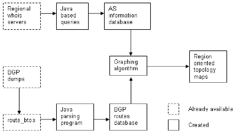
Figure 3.1 Flow chart for the topology maps creation process

The topology maps creation process has been summarized in Figure 3.1. The tools already available are shown in dashed lines, while the tools created have solid lines. The process is further analyzed in this section.

Before drawing a BGP connectivity graph, some data needs to be collected: BGP routing data and AS identification data. The collection process consists of the next steps:

1. Obtain BGP dumps from various points in RIS RIPE

(37)

3. Create a MySQL database and load the ASCII data into it. This is done via a Java based interface

4. Obtain the name and country of each AS from the regional NIC. This is done using an automated Java routine

5. Create another MySQL table for the AS specific data and load the data into it

The fourth step in the process is a difficult one due to the non-standardization for the AS data collection in the regional NICs. The Java routine uses an AS number assignation table from IANA, [25], that has the AS number range corresponding to each regional NIC. With this knowledge the program selects the “who is” server corresponding to the AS

number which data is going to obtain. The program does the query and obtains the information than is later parsed to obtain a tab separated text file.

For example, lets take the AS number 701. According to IANA this number lies in the range 1-1876 which is assigned to ARIN. The program sees this and connects to ARIN’s whois server and executes the query a 701. This results in Table 3.1:

Table 3.1 Result of querying ARIN’s whois service for AS 701

OrgName: UUNET Technologies, Inc. OrgID: UU

Address: 22001 Loudoun County Parkway City: Ashburn

StateProv: VA PostalCode: 20147 Country: US

From this result, the program obtains the name of the AS (UUNET) and the country (US) which is saved in a text file in a single line as:

701 UUNET Technologies, Inc. US

However, for other NICs, the flag OrgName might be replaced by the owner flag (like in

LACNIC’s database). The Country flag is not mandatory; in some databases this

information is located in the Address flag but not as an ISO country identifier but as the

country’s full name. In those cases, the ISO code must be obtained from the full name.

For these differences, the program must do different parsing methods for each regional NIC. This is particularly difficult in the RIPE database, which is not even consistent between its own registries. However, due to the fact that the focus is mainly in the Americas region it is not a major issue.

Now that the required information has been collected, the graphing process can begin. The graphing process uses a Java package known as JUNG (Java Universal Network Graphics) and the data previously obtained and formatted.

(38)

1. Form an array with the AS that belong to the desired graphing region selecting them from the AS data table.

2. Select from the BGP routes those which AS_PATH ends in an AS that belongs to the selected region comparing them with the array previously formed. Only routes with distinct AS_PATH are selected.

3. Create an array with all the AS that are going to be graphed. To do this, search from right to left the routes previously selected and choose the distinct AS up until the first one that doesn’t belong in the region.

4. Create a Vertices array from the previously created array.

5. Using the selected routes, create Edges between the AS up until the first one

not belonging in the region.

6. Label each node with the data from the AS data table.

[image:38.612.167.441.285.472.2]

This creates a graph which connects the nodes in the specified region with the first node outside it.

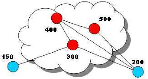
Figure 3.2 Region graph example

Consider the next example:

Let there be a set of routes

= 500 200 150 130 100 500 400 400 300 150 500 400 200 100 50 500 400 300 200 100 A

and a set B containing the AS that belong to the specific region.

B = (300 400 500)

(39)

V = (150 200 300 400 500)

[image:39.612.184.429.132.264.2]

Thus the graph would be like this:

Figure 3.3 Resulting graph from the BGP graphing algorithm

The motivation behind the third (and also the fifth) point in the algorithm comes from the way the AS_PATH is formed in the BGP process. Each AS that the announcement crosses puts its number in the AS_PATH, therefore, those AS_PATH which have as last member an AS belonging in the graphing region are those that end in it. Using this method we will obtain a graph showing the connectivity within the region and the first nodes that grant it outbound reachability.

In the previous example we have obtained a graphic showing both inbound and outbound connectivity. Inbound connectivity refers to the connections between the red nodes inside the region (shown as a cloud), while outbound connectivity refers to the connections between red and blue nodes that are outside the region.

Defining inbound connectivity as the number of neighbors directly connected to a

specified node, it is clearly seen that node 300 has an inbound connectivity of 1; 400 of 2 and 500 of 1.

Defining outbound connectivity as the sum of the reciprocal of shortest path distances

between the node inside the region and the node outside it, it is shown that 300 has an outbound connectivity of 2; 400 of 1.5 and 500 of 1.333.

3.2 Statistical Analysis of LinkRank Data

(40)

[image:40.612.93.518.68.279.2]

Figure 3.4 Flow chart for the statistical analysis of LinkRank Data

The LinkRank data analysis has been summarized in Figure 3.4. The tools already available are shown in dashed lines, while the tools created have solid lines. The process is further analyzed in this section.

For the LinkRank data 3 months have been selected for observation (July, August and September of 2006) and the prefix 12.0.1.63 that corresponds to the AS number 701 has been selected. The motivation for these selections is that a 3 month time span is sufficiently big to obtain relevant data and that the AS 701 corresponds to UUNET, a highly active and important AS.

With the obtained data a database with the following fields was built:

Table 3.2. Fields of the MySQL table containing the LinkRank data

ORIGIN Contains the prefix originating the update FROM_AS The origin AS (701)

TO_AS The destination AS (7018)

TIME The time of the change in absolute seconds DATE The date of the change

LINK The magnitude of the change

After building the database with the prefix data, the data was analyzed to obtain the most active link. This link corresponded to 701-7018 with 5878 changes in the three month time slot. AS number 7018 corresponds to AT&T, so it was not surprising that the link 701-7018 was the most active.

[image:40.612.73.568.508.597.2]

(41)

SELECT DISTINCT FROM_AS, TO_AS FROM DB WHERE FROM_AS = 701;

Resulting in:

Then a SELECT (*) COUNT was executed to each link.

[image:41.612.120.486.229.533.2]

Now that the most active link was selected the interarrival time was obtained using a Java interface. Text files with those times were created. This data was analyzed in MATLAB obtaining the following graphics:

(42)

[image:42.612.119.486.90.397.2]

Figure 3.6 Log-log plot of original data versus different models for the 701-7018 link

Both graphics show the comparison between the histogram made from real interarrival data with different models. The first graph has both axes linear while the second one is a log-log plot.

Power law in Figure 3.5, and in the following graphics, is defined by the following equation:

α

−

=x

y , (3.1)

Where = -0.7.

The exponential function is related to the statistical data from the histogram, using its mean. It is defined by the following equation:

x

e K

y µ

µ 1 1 −

(43)

The Min-square approximation is a linear regression of the data using the least squares method; it is also a power law function. It is defined by the following equation:

α β −

=e x

y . (3.3)

The coefficients for the least-squares approximation where = 3.3621 and = -1.3172.

The correlation of the data and the models is about 60% for the exponential function, while it was 93% for the power law models. From the log-log plot it can be seen that the power law is a better match for the lowest interarrival times, while the exponential gets better by the bigger times. This behavior is explained by the fact that power laws drop faster than exponential functions. Empirically it is a better model for the frequency of interarrival times, because lower times are much more frequent than higher times and the correlation coefficients obtained back up that notion.

[image:43.612.123.486.331.634.2]

The same models were applied to a different link (701-1239) obtaining similar results:

(44)

[image:44.612.123.485.90.396.2]

The least squares approximation had similar coefficients ( = 4.9528 and = -1.5548) and a correlation of 93%.

The power law behavior of interarrival times of UPDATE messages can be explained in the same manner than the power law relationship in Internet topology, or better said it is a consequence of that relationship.

As stated earlier in the “Power laws relationship in internet topology” section this behavior can be seen as a fading wave effect. When a new node joins a network it triggers a chain of restructuring changes. If we take in consideration the way UPDATE messages are created we can apply a similar reasoning.

Every time a route is advertised or withdrawn an update message is created. This event counts as a topology change, this change immediately affects its neighbors, and the change propagates to the rest of the network as a fading wave (like the ripples formed from throwing a stone into a lake).

(45)

Figure 3.9 Two interdomain nodes with high degree

Consider a withdrawn route to one of node A’s neighbors in Figure 3.9 different than B. This withdrawal will be notified to B. Given that B is highly connected it has many neighbors and given that A is also highly connected there is a high probability that many of B’s neighbors will use the A-B link to reach the withdrawn route from A, therefore, many routes will be withdrawn from the A-B link in a short period of time.

Now consider the opposite scenario, in which the withdrawn route is brought back up. In that situation the same reasoning holds. When the route is brought back up it will be notified to B. Given that B is highly connected it has many neighbors and given that A is also highly connected there is a high probability that many of B’s neighbors will use the A-B link to reach the newly announced route from A, therefore, many routes will be added to the A-B link in a short period of time.

Let us call near neighborhood the routing space formed only of A’s and B’s neighbors.

Then, we can say that routing changes in the near neighborhood will create many announcements in a short period of time.

Now, when a routing change occurs beyond the near neighborhood it will propagate slower and in minor quantity. The reasoning for this asseveration goes as follows: let us suppose a new route has been announced beyond the near neighborhood from the side of A. That change will affect only some of the neighbors of A. A will announce this change to B, but given B’s high connectivity it might have other ways to reach the new announced route besides going through A. So, not only A’s announcement is lower in quantity (fewer of A’s neighbors are affected) it also generates a lesser response from B in a bigger period of time.

(46)

As stated in [26], in the AS level topology, given the power law relationship between the node degree and rank, nodes with high degree have a really high degree. Therefore, is because of this power law topology relationship that the power law relationship for the time between changes in the number of routes in the link between two nodes with high degree also holds.

For the two other possible link cases, high degree node with low degree node (H-L link) and low degree node with low degree node (L-L link), other results were obtained. It is important to notice that an H-L relationship is defined in this work as a ratio of 20:1 or more between the degrees of the nodes. The high degree nodes analyzed in this work have around 400 neighbors. This ratio was also preferred because even when the low degree node is smaller in comparison with the high degree node, it still has enough connectivity to be significant (i.e. not being a stub relationship).

[image:46.612.123.486.328.629.2]

For the link between a high degree node and a low degree node the link 3130-1239 was analyzed, obtaining the results shown in Figure 3.10 and 3.11.

(47)

While the data approaches a power law behavior it can be seen that the probability of lower times begins low, then reaches a maximum and then follows a power law relationship.

This difference in behavior can also be explained from the topology characteristics of this link. The behavior is almost the same as in the H-H link, but the maximum has been slightly displaced to the right. One can infer that the difference in behavior is because the low degree node pulls the time to the right, however, since the high degree node has a

really high degree in comparison, it maintains the power law behavior.

[image:47.612.128.479.93.383.2]

Consider a withdrawn or added route to one of the neighbors of A different than B in Figure 3.12. A will notify B of this change, and B will notify its neighbors as well. Given A’s high degree, B has a high probability of using the A-B link to reach A’s neighbors. Therefore, the A-B link will have a change in the number of routes, but given B’s low degree it will not be as high as the change in the H-H link.

(48)

Figure 3.12 Link between a high degree node and a low degree node

The link between two low degree nodes was analyzed in a similar fashion but extending the time window to one year. However, even with a one year window, there were not enough samples to reach a definitive conclusion (400 samples for a one year window, compared to 7000 samples for a three month window).

From the results seen in Figure 3.13 and Figure 3.14, a power law is not observed. The data suggests that the times are more evenly distributed, with a tendency of being heavy-tailed.

The difference is even more evident in Figure 3.15, were we make a comparison of the statistics of the different links analyzed. There we can observe how the H-L link has a different start than the H-H links, however, it reaches the same maximum than those later and then it follows a similar pattern. For the L-L link it does not appear as a power law relationship, there is not a maximum and then a big and constant drop as in the other two configurations.

(49)

[image:49.612.140.469.89.359.2]

Figure 3.13 Original data versus different models for the 3130-7575 link

[image:49.612.140.465.418.691.2]

(50)

[image:50.612.119.486.90.393.2]

Figure 3.15 Comparison between the different link configurations

Figure 3.15 summarizes the results previously observed. The H-H and H-L links have a similar and constant behavior, while the L-L link has and erratic and not as well defined one. Reasons based on the power law relationships for AS-level topology have been given for this. With this insight we can characterize AS level link behavior as reference for future works in scalability and security issues on the interdomain level.

Given the power law relationships presented in this work, for the scalability issue we can assume certain areas of interest. Knowing that the relationship holds for H-H and H-L links we can foresee some problems in the growth of these types of links. The equipment needed to support the behavior observed, the traffic implications it has and the stress on the current protocol. For the L-L links we can’t say anything conclusive on the short term, but we can observe how the growth into an H-L or H-H link could affect. Also the implications of changing providers for L type nodes in the equipment they use. It is important to notice that the fact that the power law relationship holds for the short term in H-H and H-L links short term variations from this behavior can be observed and tackled, however that is not the case for the L-L links.

(51)

(52)

Chapter 4 Conclusions and future work

In this chapter we present the conclusions generated from this work and also, in section 4.2, the future work needed to continue this line of research.

4.1 Conclusions

In this work we have analyzed routing data from the Border Gateway Protocol (BGP) in order to obtain topology maps and power law relationships for the time between the changes in number of route in interdomain level links related, in part, to the power law relationships observed in the interdomain level topology.

From this analysis we can conclude the following:

• The manipulation of routing data from BGP dumps can generate region oriented

connectivity maps for the AS-level topology. The more data we have, the more accurate our description will be.

• Region oriented maps require additional information not present in BGP dumps,

but publicly available from the regional whois servers.

• A power law relationship was observed for the frequency of the times between the

changes in the number of routes of interdomain level links of two high degree Autonomous Systems.

• This power law relationship is consequence of the power law relationships previously observed in the AS level topology. Particularly, the relationship between the rank and degree of the AS level nodes.

• A power law relationship was also observed for the link between a high degree and low degree node, however the low degree node made the power law relationship slightly different.