Estimation of risk-neutral processes in single-factor jump-diffusion interest
rate models
L. G´omez-Valle, J. Mart´ınez-Rodr´ıguez∗
Departamento de Econom´ıa Aplicada, Facultad de Ciencias Econ´omicas y Empresariales, Universidad de Valladolid, Avenida del Valle de Esgueva 6, 47011 Valladolid, Spain.
Abstract
The estimation of the market price of risk is an open question in the jump-diffusion term structure literature when a closed-form solution is not known. Furthermore, the estimation of the physical drift has a high risk of misspecification. In this paper, we obtain some results that relate the risk-neutral drift and the risk-neutral jump intensity of interest rates with the prices and yields of zero-coupon bonds. These results open a way to estimate the drift and jump intensity of the risk-neutral interest rates directly from data in the markets. These two functions are unobservable but their estimations provide an original procedure for solving the pricing problem. Moreover, this new approach avoids the estimation of the physical drift as well as the market prices of risk. An application to US Treasury Bill data is illustrated. JEL classification: G12, G17.
Keywords: interest rates, yield curves, jump-diffusion stochastic processes, numerical differentiation, nonparametric estimation.
1. Introduction
In traditional jump-diffusion interest rate models the drift, volatility and market prices of risk are usu-ally specified as simple parametric functions for pure simplicity and tractability. Moreover, most models combine well-known parametric diffusion models with different jump size distributions. For example, Ahn and Thompson (1998) combine the square root process of Cox et al. (1985) with a constant jump size, Baz and Das (1996) and Beliaeva et al. (2008) add exponential jumps to an Ornstein-Uhlenbeck process for the short rate given by Vasiceck (1997) and so on. However, there is neither evidence nor consensus about which model is the best for accurately explaining the behaviour of interest rates. Furthermore, the functions of the models are usually chosen to obtain a closed-form solution for the pricing problem. As a result, Bandi and Nguyen (2003), Johannes (2004) and Mancini and Reno (2011) proposed nonparametric jump-diffusion models of the short rates that nest most jump-diffusion processes, but it is not possible to obtain a closed-form solution for the pricing problem. However, there are a lot of efficient numerical methods to provide accurate approximated solutions to the pricing problem.
In order to obtain the yield curves when a closed-form solution is not known, the Monte Carlo method is often used in the literature because of its simplicity and properties. When we use the Monte Carlo method, we have to estimate the drift and jump intensity of the neutral interest rate. This risk-neutral stochastic process is not observable in the markets and, therefore, in the diffusion literature the risk-neutral drift is usually obtained by estimating the drift and volatility of the instantaneous interest
∗Corresponding author
Email addresses: [email protected](L. G´omez-Valle),[email protected](J. Mart´ınez-Rodr´ıguez) Manuscript
rates and market price of risk, separately. However, this is not possible in the jump-diffusion literature. The usual absence of arbitrage argument can no longer be applied, as jump risk cannot be diversified away using traded bonds, Nawalkha et al. (2007). Therefore, it is not possible to estimate the market prices of risk unless a closed-form solution is known. In diffusion models there is another alternative which consists of estimating the risk-neutral drift directly form market data, as in G´omez-Valle and Mart´ınez-Rodr´ıguez (2008).
The main goal of this paper is to show results to estimate the drift and the jump intensity of the risk-neutral interest rates directly from market data in a jump-diffusion model. These results open up a way to solving the problem of pricing interest rate derivatives efficiently and without arbitrary restrictions regarding the functions of interest rate models. In the nonparametric jump-diffusion literature, the estimation of the market prices of risk problem has not been solved yet, but their values are arbitrary set, as in Johannes (2004). However, an incorrect specification of the market prices of risk can have dramatic consequences for derivatives valuation: see Bollen (1997) and Branger and Larsen (2013) for more details. In our approach, the market prices of risk of Wiener and Poisson processes do not have to be estimated. Furthermore, we don’t have to estimate the physical drift either, whose estimation has a high risk of misspecification.
This approach can be used for parametric as well as nonparametric models. In this paper, we use nonparametric methods such as kernel methods to avoid any arbitrary restriction in the whole model.
In order to show the finite sample properties of our approach, we make certain numerical experiments to obtain the yield curves in a test problem. Finally, we show the superiority of our approach for a nonparametric jump-diffusion term structure model with US interest rate data.
The rest of the article is organized as follows: Section 2 presents the jump-diffusion interest rate model to be studied. Section 3 shows a new approach for estimating the drift and jump intensity of the risk-neutral interest rates by means of the slope of the yield curve and zero-coupon bonds with numerical differentiation. We will call this new approach GNEJ: General Nonparametric Estimation for Jumps. Section 4 analyzes the finite sample performance of this approach using numerical differentiation and a nonparametric method. Section 5 examines empirically the behaviour of the GNEJ approach with US interest rates data. Conclusions are contained in Section 6.
2. The term structure model
In this section, we present a jump-diffusion term structure model with only one state variable. Al-though one-factor models have several shortcomings, they are still very attractive for practitioners and academics because they offer a unifying tool for the pricing of many interest rate derivatives.
Let (Ω,F,P) be a probability space equipped with a filtration F satisfying the usual conditions. The price of an interest rate security is driven by the instantaneous interest rate, which follows a mixed jump-diffusion stochastic process of the type:
dr(t) =µ(r(t))dt+σ(r(t))dW(t) +J(r(t), Y(t))dN(t), (1)
t of a zero-coupon bond maturing at time T, with t ≤ T, can be expressed as P(t, r;T). This bond is assumed to have a maturity value of one unit, i.e.:
P(T, r;T) = 1. (2)
We also assume that there exists a new measure Q, equivalent to P, such that the price of a zero-coupon bond is
P(T, r;T) =EQ
exp
−
Z T
t
r(u)du
|F(t)
, (3)
whereEQdenotes the conditional expectation under measureQwhich is known as risk-neutral probability measure. UnderQ, the short-rate r follows the process:
dr = µ(r)−σ(r)θW(r) +λQ(r)EY[J(r, Y)]
dt+σ(r)dWQ(t) +J(r, Y)dN˜Q(t),
where WQ is the Wiener process under Q, θW is the market price of risk of the Wiener process, ˜NQ
represents the compensated Poisson process, under Q measure, with intensity λQ(r) = λ(r)θN(r). For simplicity and tractability, we assume that the distribution of the jump size under Qis known and equal to distribution underP, as usual in the literature, see Das and Foresi (1996), Nawalkha et al. (2007) and Branger and Larsen (2013). That is, we assume that all risk premium related to jump risk is artificially absorbed by the change in the intensity of jump from λ under the physical measure to λQ under the risk-neutral measure.
In the absence of the jump component, it is possible to derive the term structure equation by con-structing a riskless portfolio of two bonds of different maturities and imposing the absence of the arbitrage condition. However, in the presence of a jump component, the absence of arbitrage argument can no longer be applied, as jump risk cannot be diversified away using traded bonds, Nawalkha et al. (2007). Therefore, the valuation of fixed income securities requires transition from actual to the equivalent mar-tingale measure. In general, this task can be accomplished by specifying a stochastic discount factor for the economy and can be used directly to obtain the term structure equation consistent with the process given in (1). Thus, the pricing partial integro-differential equation is as follows:
Pt(t, r) + µ(r)−θW(r)σ(r)
Pr(t, r) + 1 2σ
2(r)P
rr(t, r)−rP(t, r)
+ λQ(r)EY[P(t, r+J)−P(t, r)] = 0, (4)
see Nawalkha et al. (2007). This pricing equation is the same for all interest rate derivatives we only have to add the corresponding final conditions. In order to obtain the term structure: µ, σ,θW,λQ must
be estimated. Then, these functions are replaced in the pricing equation (4) and this is solved by taking into account the final condition (2).
Finally, the yield curve can be expressed as:
R(t, r;T) = −ln(P(t, r;T))
T −t . (5)
3. Exact results and approximations
(2003) and Johannes (2004) show how to estimate µ,σ and λ by means of moment equations with data in the markets. However, this approach does not allow us to estimate the market prices of risk, which are necessary to price interest rate derivatives but they are not observable. Therefore, we propose a novel approach for estimating efficiently the coefficients of the pricing partial integro-differential equation (4) directly from the data. We estimate the risk-neutral drift and the risk-neutral jump intensity without estimating the market prices of risk. In order to apply this approach, we prove the following results which relate the drift and jump intensity of the risk-neutral interest rates directly to the prices and yields of zero-coupon bonds.
Theorem 1. Let P(t, r;T) be a solution to (4) subject to (2), and r follows a jump-diffusion stochastic process given by (1), then:
∂R ∂T|T=t =
1
2 µ(r)−σ(r)θ W
(r) +λQ(r)EY[J(r, Y)]
. (6)
We prove this result by means of the Feynman-Kac solution in (3). The detailed proof of this theorem can be found in the Appendix. An analogous result, although for just a diffusion process, is also shown in G´omez-Valle and Mart´ınez-Rodr´ıguez (2008).
This theorem can be very useful. According to (6) the risk-neutral interest rate drift, which is the basis for the general asset pricing theory, is equal to the slope of the yield curve close to maturity. This result allows us to estimate the risk-neutral interest rate drift, which is unobservable, from yields of zero-coupon bonds.
Theorem 2. Let P(t, r;T) be a solution to (4) subject to (2), and r follows a jump-diffusion stochastic process given by (1), then:
∂(r2P)
∂T |T=t=−r
3(t) + 4r(t)∂R
∂T|T=t+σ
2(r) +λQ
(r)EY[J2(r, Y)]. (7)
We prove this result with a similar technique to Theorem 1. This proof can be found in the Appendix. This theorem allows us to estimate the risk-neutral jump intensity of the interest rate by the prices of zero-coupon bonds and the slope of the yield curve.
At this point it is important to note that with our approach we have to estimate 4 functions instead of 6. This fact obviously reduces the high computational cost of jump-diffusion models and, therefore, they become more attractive for practitioners. Moreover, we do not have to estimate either the market prices of risk of Wiener and Poisson processes, which are not observable, or the physical drift of the interest rate, which has more risk of misspecification than volatility: see Chapman et al. (2001). Therefore, the GNEJ approach allows us to reduce the misspecification errors.
In order to implement these theorems we rely on numerical differentiation. We use yields of zero-coupon bonds at points that are inside the time interval to approximate the slope at the boundary of the time domain. More precisely, we apply a second order forward difference formula to obtain greater accuracy of (6), with a step size ∆>0, see Burden and Faires (2001):
∂R ∂T|T=t =
−3R(t, t) + 4R(t, t+ ∆)−R(t, t+ 2∆)
2∆ +O(∆
2
), (8)
Finally, it is important to observe that any parametric or nonparametric technique can be applied to estimate the slopes. In this paper, we use the Nadaraya-Watson nonparametric estimator. Suppose a data-set consists of N pairs of observations, (r1, X1),· · ·,(rN, Xn), where ri is the explanatory variable and Xi is the response variable. We assume a model of the kind Xi =g(ri) +i, whereg(r) is a unknown function andiis an error term, representing random errors in the observations or variability from sources not included in the ri. The errori are assumed to be independent and identically distributed with mean 0 and finite variance. The estimate has the closed form
ˆ
g(r) =
PN
i=1wi(r)Xi
PN
i=1wi(r)
, (9)
wherewi(r) =K(r−hri) are weight functions (for example the Gaussian kernel which is widely used in the literature and we use it in this paper) and h the bandwidth, see H¨ardle (1999).
4. Numerical experiments
In this section, we show the robustness of this technique by obtaining the yield curves. Note that we can price in the same way any other interest rate derivatives by solving the identical equation and considering another different boundary condition.
We investigate the finite sample performance of the GNEJ approach using a test problem in a non-parametric setting and the Monte Carlo method.
As a basic test problem, we consider a jump extended square root process with exponential jumps which is denoted as CIR-EJ:
dr =β(m−r)dt+σ√rdW(t) +Y(η)dN(t),
where the jump size, Y, is an exponential random variable with an expected value η. The market prices
of risk are as follows: θW(r) = θ
σ
√
r, θN = ϕ, see Nawalkha et al. (2007) for more details. The only reason we choose this model is because a closed-form solution is known and therefore we can obtain the true risk-neutral drift, risk-neutral jump intensity and the exact yield curves to make comparisons.
In our implementation, we assume that the market prices of risk parameters are: θ = −0.167 and
ϕ = 0.5, which are coherent with the values in the literature. Next, we combine them with the values of the parameters used by Beliaeva and Nawalkha (2012) to price zero-coupon bonds and bond options. Therefore, we assume that: β = 0.267, m= 0.03, σ = 0.075, λ= 2, η = 0.01.
For series generation, we use the Euler-Maruyama stochastic differential equation discretization scheme, Platen and Bruti-Liberati (2010), an explicit order 0.5 strong and order 1.0 weak scheme. We discard the burn-in period (the first part of the whole series) to avoid the starting value effect. In all the numer-ical experiments we simulate 5000 sample paths with a time interval ∆t = 1/250, that is to say, daily observations, and a realization length N = 7500, which is equivalent to 30 years of daily observations.
In order to make comparisons, we obtain the exact yield curves obtained with the CIR-EJ model and the approximated yield curves with the moment equations technique and the GNEJ approach.
First, we use the moment equations proposed by Bandi and Nguyen (2003) and Johannes (2004):
M1(r) = lim
∆t→0E[r(t+ ∆t)−r(t)|F(t)] =µ(r) +λ(r)EY[J], (10)
M2(r) = lim
∆t→0E[r(t+ ∆t)−r(t))
2|F(t)] =σ2(r) +λ(r)E
Y[J2], (11)
Mk(r) = lim
∆t→0E[r(t+ ∆t)−r(t))
k|F(t)] =λ(r)E
see Bandi and Nguyen (2003) for regularity conditions and limiting distributions. These limiting moment conditions extend the well-known instantaneous moment conditions of a diffusion.
In our test problem, we have assumed that J(r, Y) = Y and the jump size Y is distributed exponen-tially with a positive mean η, Y Exp(η). Thus,
EY[Yk] =ηkk!, k= 1,2,3, . . . (13)
We replace (13) in (10)-(12) and obtain the moment conditions necessary to estimate the interest rate coefficients for the CIR-EJ process. See Bandi and Nguyen (2003) and Johannes (2004) for a similar approach but with other jump size distributions.
To estimate the conditional moments, we use the Nadaraya-Watson estimator1, as in Johannes (2004).
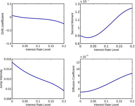
Figure 1 reports pointwise averages for fits of the nonparametric estimated functions over the 5000 simulations. The upper left panel gives the drift estimation results and the top-right panel plots the instantaneous second moment. If the data were generated by a single factor diffusion model, the second moment would estimate the diffusion coefficient. However, in jump-diffusion models, the second moment estimates σ2(r) + 2η2λ(r). The lower-left panel reports estimates of the intensity jump, scaled to daily
units. Finally, the bottom-right panel plots the diffusion coefficient estimates. The estimation ofσ2(r) is
more difficult because it depends on three other estimates (the jump mean, the jump intensity and the second moment), which magnifies any sampling error. The point estimate of η is 8.8308×10⁻³.
0 0.05 0.1 0.15 0.2 −0.4
−0.2 0 0.2
Interest Rate Level
Drift coefficient
0 0.05 0.1 0.15 0.2 0.8
0.9 1 1.1 1.2 1.3x 10
−3
Interest Rate Level
Second Moment
0 0.05 0.1 0.15 0.2 0.008
0.01 0.012 0.014 0.016
Interest Rate Level
Jump Intensity
0 0.05 0.1 0.15 0.2 2
4 6 8 10 12
x 10−4
Interest Rate Level
Diffusion Coefficient
Figure 1: Nonparametric drift, second moment, jump intensity and diffusion estimations with the moment equations approach for a jump-diffusion model with exponential jump. In each pane, we show the pointwise mean across the 5000 simulations with the moment equations. In all the cases the simulation length is 7500 and the length of time between observations ∆t= 1/250.
1The choice of the optimal bandwidth is elusive in the literature. We use h
However, there are still other functions to be estimated: the market prices of risk. In the diffusion term structure literature, this function is estimated by means of a no-arbitrage argument as in Stanton (1997) but this is not valid in jump-diffusion models, Nawalkha et al. (2007). Moreover, to the best of our knowledge, the estimation of the market prices of risk in jump-diffusion is an open question in the term structure literature when a closed-form solution is not known. Johannes (2004) assumes that the market price of risk of the Wiener process is zero, because in Stanton (1997) this value was small. As far as the market price of jump risk is concerned, Johannes (2004) assumes different parameters which are arbitrary chosen, for example equal to one. This means that the jump intensity is equal to the risk-neutral jump intensity: λQ =λ. In order to be able to make comparisons with the GNEJ approach, we also consider both assumptions to price zero coupon bonds with the moment equation approach, although we think that these assumptions are not accurate.
In order to apply the GNEJ approach, we rely on the results obtained in the previous section: The-orems 1 and 2, numerical differentiation and (9) with the Nadaraya-Watson2 estimator and Gaussian kernel. First, we estimate the risk-neutral drift from (6) by means of the second order approximation (8). To be exact, we use yields with maturities of 6 months and 1 year in order to estimate the slope of yield curve. Finally, we replace the EY[J2] and σ2, which have been previously estimated with the moment equations approach, in (7) to estimate the risk-neutral jump intensity, λQ, by means of a second order approximation and yields and prices with maturities of 6 months and 1 year in a similar way to the slope of yield curve.
Note that the drift and the market prices of risk of the Wiener and Poisson processes do not have to be identified or estimated with this approach, because the risk-neutral drift and jump intensity are estimated directly from interest rate data.
Throughout this paper, in order to analyze the behaviour of our approach, we always use the root
mean square error: RMSE =
q
1
N
PN
t=1(R(t)−Rˆ(t))2, where N is the number of observations, R(t) is
the observed or theoretical value and ˆR(t) is the estimated value with the corresponding model.
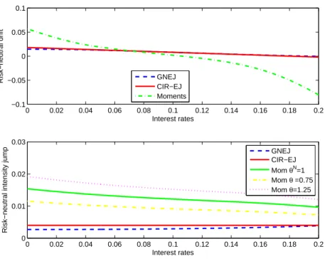
Figure 2 upper panel shows the true and pointwise averages for fits of the risk-neutral drift of the interest rates using the GNEJ and the moment equations approaches. The fitted risk-neutral drift using the GNEJ approach is very similar to the exact risk-neutral drift and the differences are small. This gives as a result a low RMSE, which is equal to 1.0409×10⁻³. However, the risk-neutral drift using the moment equations is very different. The differences are quite important for nearly all interest rate levels, specifically in this case the RMSE is equal to 2.7873×10⁻². This fact is mainly due to the poor
estimation of the drift and especially of the market price of risk of the Wiener process.
Figure 2 bottom panel shows the true and pointwise average for fit of the risk-neutral intensity jump, scaled to daily units, using the GNEJ and moment equations approaches. The fitted risk-neutral jump intensity using the GNEJ approach is quite similar to the exact one. This gives as a result a low RMSE, which is equal to 1.0344×10⁻³. However, the risk-neutral jump intensity obtained with the moment
equations changes considerably with the value that we impose to the market price of risk of the Poisson process. If we consider θN = 1, the RMSE is considerably higher: 8.4255×10⁻³. In order to make comparisons we also assume different values for the market price of risk of the Poisson process, as in Johannes (2004). For example, if θN = 1.25 the RMSE increases to 1.1517×10⁻². If we consider lower
values, for example, θN = 0.75 the RMSE decreases to 5.3379×10⁻³. However, there is no approach to obtain theθN that minimizes the RMSE. Moreover, if we have real data, the risk-neutral jump intensity is even unobservable. Finally, we obtain the yield curves and we compare the RMSE for different maturities.
0 0.02 0.04 0.06 0.08 0.1 0.12 0.14 0.16 0.18 0.2 −0.1
−0.05 0 0.05 0.1
Interest rates Risk−neutral drift GNEJ
CIR−EJ Moments
0 0.02 0.04 0.06 0.08 0.1 0.12 0.14 0.16 0.18 0.2 0
0.01 0.02 0.03
Interest rates
Risk−neutral intensity jump
GNEJ CIR−EJ Mom θN=1
Mom θ =0.75 Mom θ=1.25
Figure 2: The true risk-neutral drift and jump intensity for the CIR-EJ model and the nonparametric estimation results with the GNEJ and moment equations approaches. We show the pointwise mean across the 5000 simulations with the GNEJ and moment equation approaches. In all the cases the simulation length is 7500 and the length of time between observations ∆t= 1/250.
Table 1: RMSE with the different approaches for the 5000 simulated yield curves withN = 7500 and ∆t= 1/250.
6 Months 9 Months 12 months 18 Months 24 Months Moment 9.622×10⁻³ 1.406×10⁻² 1.765×10⁻² 2.451×10⁻² 3.041×10⁻²
GNEJ 7.972×10⁻⁴ 1.129×10⁻³ 1.431×10⁻³ 1.796×10⁻³ 2.053×10⁻³
In order to price zero-coupon bonds we have to solve the pricing equation (4) subject to (2). However, when nonparametric methods are used it is not possible to find a closed-form solution and a numerical method must be applied to obtain an approximated solution. Therefore, we apply the Monte Carlo method with 10000 simulations and a discretization interval equal to one day. The number of simulations and the discretization interval are chosen to render the Monte Carlo error negligible: see Johannes (2004). Figure 3 displays a comparison between the true yield curves with the CIR-EJ model and those estimated with the moment equations and GNEJ approaches for different interest rate levels. In all the cases the yield curves obtained with the GNEJ approach are closer to the exact ones than those obtained with the moment equations technique.
Table 1 shows the performance of the GNEJ and the moment equations approach to obtain the yield curves for different maturity times. Note that the GNEJ approach provides lower errors than the moment equations technique for all the maturities. In fact the errors of the GNEJ approach are approximately up to one order of magnitud lower than the errors of the traditional technique.
6m 9m12m 18m 24m 36m 0.02
0.03 0.04 0.05 0.06
Maturity time
R
r=0.03
6m 9m12m 18m 24m 36m 0.06
0.07 0.08 0.09
Maturity time
R
r=0.05
6m 9m12m 18m 24m 36m 0.06
0.08 0.1 0.12 0.14
Maturity time
R
r=0.11
6m 9m12m 18m 24m 36m 0.1
0.12 0.14 0.16
R
r=0.15
Maturity time GNEJ
Moments CIRJ
Figure 3: Yield curves for different interest rate levels. The yield curves are obtained with the GNEJ and the moment equations approaches for the CIR-EJ model. In all the cases we use the pointwise average over the 5000 simulations, with a simulation length of 7500 and length of time between observations ∆t= 1/250
Table 2: Summary of the statistics of the US 3-month Treasury Bill rates and the first differences, January 1971 to February 2013.
Variable N Mean Std. dev. Max. Min.
rt 10519 5.279×10⁻² 3.323×10⁻² 1.752×10⁻¹ 1.0×10⁻⁴ rt+1−rt 10518 −4.592×10⁻⁶ 1.067×10⁻³ 1.393×10⁻² −1.321×10⁻²
5. Data and empirical analysis
In this section, we implement the GNEJ approach with US interest rates data to reexamine the pricing of yield curves in jump-diffusion models. We compare the results obtained with the GNEJ approach to the moment equations technique and we show that the GNEJ approach outperforms it.
The short rate is inherently unobservable, and it has to be approximated using interest rates of short term zero-coupon bonds: Chapman et al. (2001) for a detailed discussion. In this paper we use the 3-month Treasury Bill rates because Mancini and Reno (2011) showed that any instrument with maturity below three months should not be used when estimating jump-diffusion processes.
Data were obtained from the Federal Reserve h.15 database. Daily rates were converted from discounts to annualized interest rates and no specific adjustments were made for weekends or holidays. The sample period covers from January 1971 to February 2013. Table 2 summarizes the data.
the 1-year Treasury Bill for the whole estimation period of time.
First, we obtain the yield curves using the GNEJ approach as in Section 4 but we assume two different jump size distributions,Y: exponential and normal, which are very common in the interest rate literature. In the numerical experiments in Section 4, we assumed that the jump size was distributed only exponentially because in that case a closed-form solution was known and this fact is necessary to have a test problem. If we assume that the jump size is normal, Y N(0, σ2
Y), we will use the normal moments in Bandi and Nguyen (2003):
EY[Y2k] =σY2k k
Y
n=1
(2k−1), (14)
EY[Y2k−1] = 0, k= 1,2,3, . . . , (15)
to estimate σ2 and E
Y[J2].
All the estimations are done using the Nadaraya-Watson3 estimator in (9), as in Johannes (2004).
0 0.02 0.04 0.06 0.08 0.1 0.12 0.14 0.16 0.18 0.2
0.005 0.01 0.015 0.02 0.025 0.03 0.035 0.04
Interest rates
Risk−neutral drift
GNEJ 95% conf. Bands
0 0.02 0.04 0.06 0.08 0.1 0.12 0.14 0.16 0.18 0.2
0 0.5 1 1.5
2x 10
−6
Interest rates
Risk−neutral jump intensity
GNEJ 95% conf. Bands
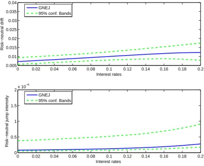
Figure 4: The estimated risk-neutral drift and risk-neutral jump intensity and 95% confidence bands using 10000 iterations of the Kunsch (1989) block bootstrap algorithm.
Figure 4 shows the estimated risk-neutral drift and jump intensity, scaled to daily units, jointly with the 95% confidence bands calculated using the block-wise bootstrap algorithm of Kunsch (1989). In both cases, the estimated functions are between the confidence bands although when interest rates are very high the difference increase slightly.
In order to obtain the yield curves we have to solve the pricing equation (4) subject to (2). We use the Monte Carlo method with 5000 simulations and a discretization interval equal to one day. Table 3 shows the RMSE of the yield curves when the jump size follows a normal and exponential distribution.
3We useh
r=hσr as bandwidth, with the smoothing parameterh= 1.2 for the second moment andh= 1.5 for higher
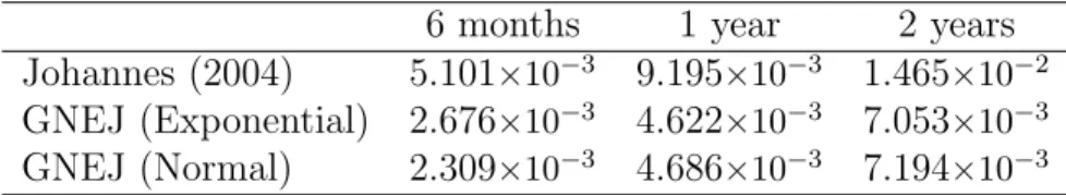
Table 3: The RMSE of the yield curves for different maturity times.
6 months 1 year 2 years
Johannes (2004) 5.101×10⁻³ 9.195×10⁻³ 1.465×10⁻²
GNEJ (Exponential) 2.676×10⁻³ 4.622×10⁻³ 7.053×10⁻³
GNEJ (Normal) 2.309×10⁻³ 4.686×10⁻³ 7.194×10⁻³
In all the cases and for all the range of maturities, the errors are very similar and the order of accuracy is 10−3.
Finally, in order to gauge the performance with the models considered in the literature, we also obtain the yield curves using the Johannes (2004) model4. He assumes that the jump intensity is lognormal and estimates all the functions with the moment equations. As far as the market prices of risk is concerned we also consider, as Johannes (2004), that the market price of risk of the Wiener process is zero and the market price of risk of the Poisson process is equal to one. Notice, that Johannes (2004) assumes these values arbitrarily because there is not any approach to estimating them when a closed-form solution of the model is not known.
In Table 3, we also show the RMSE of the model proposed by Johannes (2004) and we see that the errors are considerably higher than with the GNEJ approach. They are about twice as high for all the maturity range.
Therefore, the results in this section also confirm the superiority of the GNEJ approach for obtaining the yield curves in a nonparametric term structure model with real data.
6. Conclusions
In order to price interest rate derivatives with jump-diffusion processes, we provide a novel procedure based on the estimation of the drift and jump intensity of the risk-neutral interest rates. This technique is notable because neither the physical drift nor the market prices of risk have to be estimated. As a consequence, it is not necessary to make arbitrary assumptions about the market prices of risk as usual in the literature where a closed-form solution is not known. Furthermore as we estimate the risk-neutral drift directly form the data in the market we reduce the misspecification error because we don’t have to estimate the physical drift. Finally, this approach is adaptable: both parametric and nonparametric methods can be used to estimate the required functions.
We show the practical interest of this new approach in an empirical experiment with US Treasury Bill data.
Acknowledgements
This work was supported in part by the project VA191U13 of the Junta de Castilla y Le´on and the GIR Optimizaci´on Din´amica, Finanzas Matem´aticas y Utilidad Recursiva of the Universidad de Valladolid. J. Mart´ınez-Rodr´ıguez was also supported in part by the project of the Ministerio de Ciencia e Innovaci´on MTM2011-25138
4We use similar smoothing parameters than Johannes (2004), that is, h= 1.25 for the first moment and h= 0.4 for
Appendix
In this appendix, we prove the Theorems 1 and 2 in Section 3.
Proof of Theorem 1.
Let Z be the Radon-Nikodym derivative of Q with respect to P. Then, we can define the Radon-Nikodym derivative process as:
Z(t) =E[Z|F(t)], 0≤t≤T.
This process verifies:
dZ(t) = Z(t)[−θWdW(t) + (θN −1)dN˜(t)],
see Runggaldier (2003). We denote the compensated Poisson process ˜N, the discount process D(t) =
−Rt
0 r(s)ds and we havedD=−rDdt. Then, we obtain:
d(ZD) =ZD[−rdt−θWdW + (θN −1)dN˜].
Taking into account that EQ[D(T)|F(t)] = 1
Z(T)E[Z(T)D(T)|F(t)],
P(t, r;T)−P(t, r;t) = E[−r(T)Z(T)D(T)|F(t)].
Changing the order of the integral, Billingsley (1995), and calculating the derivative:
∂P
∂T(t, r;T) =E[−r(T)Z(T)D(T)|F(t)] =−r(T)P(t, r;T).
Therefore:
∂2P
∂T2(t, r;T) =
∂
∂T(−r(T)P(t, r;T)). (A.1)
On the other hand:
d(rZD) = ZD[(−r2+ (µ−σθW) +λθNEY[J])dt + (σ−rθW)dW + (r(θN −1) +J θN)dN˜].
Once more, we change the order of the integral, Billingsley (1995), and we calculate the derivative:
∂(rP)
∂T (t, r;T) = (−r
2(T) + (µ(r)−σ(r)θW(r)) +λ(r)θN(r)E
Y[J(r, Y)])P(t, r;T).
Then we can write
∂(rP)
∂T |T=t=−r
2(t) + (µ(r)−σ(r)θW(r))+λ(r)θN(r)E
Y[J(r, Y)],
and from (A.1) and λQ =λθN:
∂2P
∂T2|T=t=r 2
This results in (6).
Proof of Theorem 2.
By means of (A.2) we also have:
d(r2ZD) = ZD[(−r3+ 2r(µ−σθW) + 2rλθNEY[J] +λθNEY[J2] +σ2)dt + (2rσ−r2θW)dW + (µrθNJ +r2(θ−1) +θNJ2)dN˜].
Analogously to the proof of Theorem 1, we obtain:
∂(r2P)
∂T (t, r;T) = P(t, r;T)
−r3(T) + 2r(T)(µ(r)−σ(r)θW(r))
+2r(T)λQ(r)EY[J(r, Y)] +λQ(r)EY[J2(r;Y)] +σ2(r)
.
Then, by (6) we obtain (7).
Bibliography
Ahn, C., Thompson, H., 1998. Jump-processes and the term structure of interest rates. The Journal of Finance 43, 155-174.
Bandi, F.M., Nguyen, T.H., 2003. On the functional estimation of jump-diffusion models. Journal of Econometrics 116 , 293-328.
Baz, J., Das, S.R., 1996. Analytical approximations of the term structure for jump-diffusion processes: a numerical analysis. The Journal of Fixed Income 6, 78-86.
Beliaeva, N., Nawalkha, S.K., Soto, G., 2008. Pricing American interest rate options under the jump-extended Vasiceck model. The Journal of Derivatives 16 , 29-43.
Beliaeva, N., Nawalkha, S.K., 2012. Pricing American interest rate options under the jump-extended constant-elasticity-of-variance short rate models. Journal of Banking and Finance 36 , 151-163.
Bollen, N.P.B., 1997. Derivatives and the price of risk. The Journal of Futures Markets 17, 839-854.
Branger, N., Larsen, L.S., 2013. Robust portfolio choice with uncertainty about jump and diffusion risk. Journal of Banking and Finance 37, 5036-5047.
Burden, R.L., Faires, J.D., 2001. Numerical Analysis, Brooks/Cole Publishing Co, Seventh edition.
Billingsley, P., 1995. Probability and Measure, Wiley Series in Probability and Mathematicaal Statistics, Third edition.
Chapman, D., Long, J., Pearson, N., 2001. Using proxies for the short rate: When are three months like an instant? Review of Financial Studies 12, 763-806.
Cox, J.C., Ingersoll J.E., Ross S.A., 1985. A theory of the term structure of interest rates. Econometrica 53, 385-407.
G´omez-Valle, L., Mart´ınez-Rodr´ıguez, J., 2008. Modelling the term structure of interest rates: An efficient nonparametric approach. Journal of Banking and Finance 32, 614-623.
H¨ardle, W., 1999. Applied nonparametric regression. In: Econometric Society Monographs, vol. 19. Cambridge University Press, New York.
Hong,Y., Li, H., 2005. Nonparametric specification testing for continuous-time models with applications to term structure of interest rates. Review of Financial Studies 18, 37-84.
Jiang, G.J., 1997. A generalized one-factor term structure model and pricing of interest rate derivative securities. University of Grominger. Research report.
Johannes, M., 2004. The statistical and economic role of jumps in continuous-time interest rate models. The Journal of Finance 59, 227-259.
Kunsch, H.R., 2004. The jacknife and the bootstrap for general stationary observations. Annals of Statis-tics 17, 1217-1241.
Mancini, C., Reno, R., 2011. Threshold estimation of jump-diffusion models and interest rate modeling. Journal of Econometrics 160, 77-92.
Nawalkha, S.K., Beliaeva, N., Soto, G., 2007. Dynamic Term Structure Modeling. John Wiley & Sons, Inc.
Øksendal, B., Sulem, A., 2005. Applied Stochastic Control of Jump Diffusions. Springer-Verlag, Berlin, Heidelberg.
Platen, E., Bruti-Liberati, N., 2010. Numerical Solution of Stochastic Differential Equations with Jumps in Finance. Springer-Verlag, Berlin Heidelberg.
Runggaldier, W.J., 2003. Jump-Diffusion Models. Handbook of Hevay Tayled Distributions in Finance. S.T. Rachev, Universitat Karisruhe, Karisruhe, Germany, North Holland, 169-209.
Shreve, S.E., 2004. Stochastic Calculus for Finance II: Continuous Time Models. Springer Finance, New York.
Stanton, R., 1997. A nonparametric model of term structure dynamics and the market price of interest rate risk. The Journal of Finance 52, 1973-2002.